Optical speed sensor with estimation of power output for a basic indoor cycling trainer (AKA poor mans smart trainer)
by Jan Heczko (jheczko@ntis.zcu.cz, jan.heczko@gmail.com)
2022-01-26
It is an almost universally accepted fact now that using a powermeter in training (and racing) helps cyclists to achieve desired performance ([TRWPM], [DJPM]). I already spent some time considering a purchase of one. This led me to thoughts on the principles of powermeter working. Being rather short of money, I also considered building a powermeter myself. Although this might not be an easy task (consider e.g. the struggles of the IQ2 startup [IQ2]) it should not be completely impossible [ERY], [JWY]. I already successfully built an MTB powermeter using the SG53 module by Sensitivus [DIYPM] - see [EAN] for the result. This text describes a somewhat overlapping effort of mine to convert a cheap[est] cycling indoor trainer into a device that would output speed, distance and perhaps an estimate of power.
NOTE: This is a work in progress and these notes are mostly meant to remind me of how I did the things. Please forgive missing parts and inconsistencies.
Contents
Operating principle
My first indoor training sessions brought to me the observation/hypothesis that there is a unique relationship between speed and the power needed to hold that speed constant. So my first thoughts were:
- To mount a classic speed sensor to my rear wheel in order to measure speed. This way I could guess my training zones based on speed instead of power.
- To put a stroboscope onto the flywheel with patterns for two or three target speeds.
The obvious problem with the two approaches emerged immediately: The relationship between power and speed is most probably nonlinear, therefore the usual setup of training zones in terms of speed wouldn't be straightforward. So although it would be possible to use speed as a measure of training intensity, it would basically require to measure the speed-power relationship. Some resources are already available for that. PowerCurve offers a sensor that turns basic indoor trainer to a power based one [PCS]. A reference to PowerCurve together with additional insight and problems of this approach are given in an answer at stackexchange [SX]. Vpower converts the output of a speed sensor into power and sends it using ANT+ to your head-unit [VPOWER].
My understanding of the above solutions is, however, that they only use the quasi-static speed-power relationship (it is explicitly stated in [VPOWER], but I only guess in the case of [PCS]). Considering the dynamic effects (inertia of the trainer+bike system) not only makes the measurement more accurate, especially in the case of short intervals or other speed changes, but also enables easy calibration. The governing equation of the quasi-static case is simply
where P is power and v stands for speed, i.e. power is a function of speed. With the consideration of inertia, one can use the motion equation (using generalized coordinates)
where F is the generalized force acting on the system, m is the reduced mass (inertia of the traner+bike system), a stands for acceleration, and FT is the generalized force-speed function. The quasi-static case may be obtained assuming a = 0:
It is however necessary, to determine speed and acceleration in order to employ the above stated equation. I used an optical gate to measure time between light pulses.
Calibration
In order to determine the parameters m and FT of the motion equation, I considered two loading cases:
- Coasting, during which the applied force is zero, F = 0.
- Acceleration by a known force F = const. I used a known weight m1 connected to the trainer+bike system by a string, led through a pulley, and forced downwards by gravity.
The first loading case (coasting) is used to determine the trainer's resistance relative to reduced mass as a function of speed, (FT)/(m)(v). To do this, one has to convert the measured data (time deltas) to an acceleration-speed relationship, a(v). The resistance relative to reduced mass is then (see Appendix 1)
This relationship is then used to obtain the reduced mass using the second loading case (acceleration by a known force). Again, the measured data (time deltas from the other set of measurements) must be converted to speed and acceleration (see Appendix 2).
I used quadratic polynomial for (FT)/(m)(v) in the numerical implementation, i.e.
Tire pressure
TBA
Temperature dependence
The three main sources of temperature dependence of the trainer's resistance are:
- Change in tire pressure and the corresponding change in rolling resistance (see e.g. [RR]).
- Change in the resistance of the trainer's break [SX].
- Change in the mechanical properties of rubber. (?)
To do: Test the influence of
- tire temperature,
- break temperature.
Notes:
- Employ cooling fan pointed toward the component(s) that should have constant temperature (but measure both!).
- Ensure that/whether temperature changes are consistent with the ideal gas law [GasLaw].
Changes in pressure should thus be proportional to temperature changes if the corresponding volume changes are negligible.
Electronics
I bought an LTH 301-07 opto-gate and built a circuit based on the information at [MCE]. There I found a working scheme and resistance values for use with an Arduino board. I used a Raspberry Pi, since I had two of them lying round, and its GPIO pins for connecting the circuit (namely the 3V3 pin, Ground pin, and ce1 pin (#17), see [GPIO]).
I did the initial testing using a breadboard. However, the cables came loose during harder riding, so I soldered the circuit using a universal circuit board.
Software
Python showed to be a viable solution together with the pigpio library [pigpio]. Registering the pulses and saving the data is done using a callback function:
import pigpio

last = [None]
cb = [None]

def get_cbf(file_name):
    def _cbf(gpio, level, tick):
        if last[0] is not None:
            diff = pigpio.tickDiff(last[0], tick)
            print(f'G={gpio} l={level} d={diff}')
            with open(file_name, 'ab') as tf:
                tf.write(struct.pack('d', diff)
        last[0] = tick

    return _cbf

def main(pin=17, filename='time_deltas.dat'):
    pi = pigpio.pi()

    if not pi.connected():
        exit()

    cb[0] = pi.callback(pin, pigpio.RISING_EDGE, get_cbf(filename))

    try:
        while True:
            time.sleep(.1)
    except KeyboardInterrupt:
        print('\nTidying up')
        for c in cb:
            c.cancel()

    pi.stop()
The struct module from the standard python library is used in order to keep the size of data files minimal.
This way, each time-delta measurement only takes 8 bytes.
Reading from the file is done similiarly:
with open(file_name, 'rb') as tf:
    dts = tf.read()

time_deltas = struct.unpack(
    'd' * (len(dts) // struct.calcsize('d')), dts)
NOTE: The above code shows the basic principle, the actual code includes power calculation and bluetooth communication.
Power calculation
The time deltas (a [numpy] array of predefined number of float values) are used to evaluate the speed and acceleration:
def get_speed_and_acceleration_avg(
        time_deltas,
        speed_const = .139 / 2,
):
    speeds = speed_const / time_deltas
    accs = (speeds[2:] - speeds[:-2]) / (
        time_deltas[2:] + time_deltas[:-2])
    avg_speed = np.mean(speeds)
    avg_acc = np.mean(accs)
    return avg_speed, avg_acc
where speed_const is the distance between two pulses and time_deltas is a chosen number of data points.
The power is evaluated using a previously calibrated polynomial:
FTM_COEFS = [-5.17781e-3, .38950767, .71346973, -.71051168]
REDUCED_MASS = 7.5
def default_resistance(speed):
    """speed in [m/s]"""
    return np.polyval(FTM_COEFS, speed) * REDUCED_MASS

def get_power(
        speed, acceleration,
        resistance_function=default_resistance,
        mass=REDUCED_MASS,
):
    return resistance_function(speed) + mass * acceleration * speed
Cadence estimation
To do - using speed fluctuations.
Bluetooth Low Energy (BLE) connection
BlueZ [BlueZ] and bluezero [bluezero] used, works with IpBike [IpBike], does not work with Garmin Edge 130.
Enclosure
The housing for the electronics is 3D printed (but a piece of wood/plastic/... would also do the job) and mounted to the body of the trainer using zip ties. Its main design objectives were to stay in place and to hold the opto-gate close to the trainer's flywheel. A rotor is glued to the flywheel so that it periodically blocks or opens the opto-coupler.
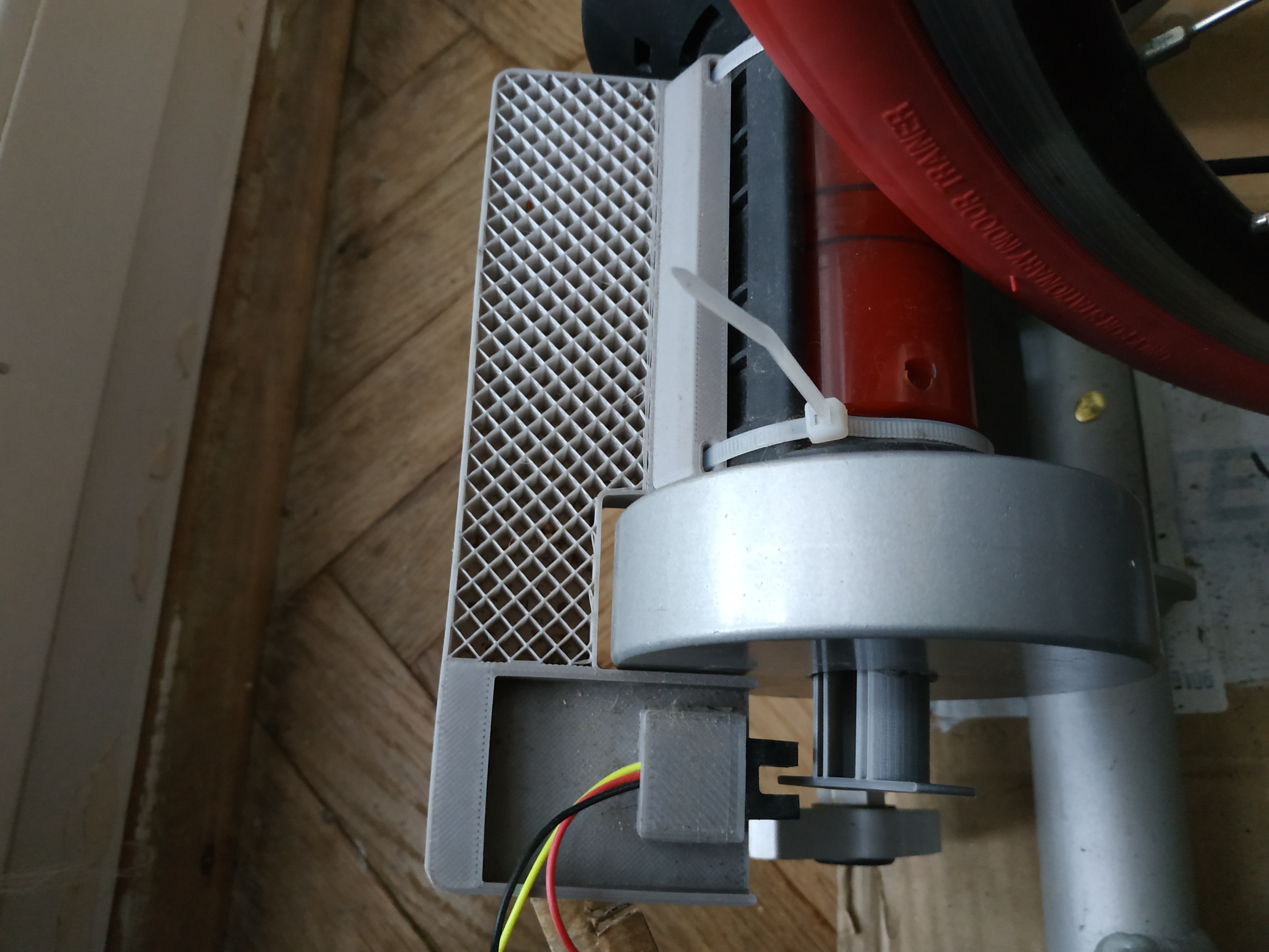
The speed sensor, mounted on the trainer.
References
| [TRWPM] | <https://www.velopress.com/books/training-and-racing-with-a-power-meter/> |
| [DJPM] | <https://www.youtube.com/c/DylanJohnsonCycling/search?query=power%20meter> |
| [IQ2] | <https://www.youtube.com/watch?v=9f7nhnwB_oM> |
| [JWY] | <https://www.youtube.com/user/kwakeham/search?query=power%20meter> |
| [ERY] | <https://www.youtube.com/c/EdROran/videos> |
| [DIYPM] | <https://sensitivus.com/products/diy-power-meter/> |
| [EAN] | <http://home.zcu.cz/~jheczko/pt.pdf> |
| [PCS] | (1, 2) <http://www.powercurvesensor.com/cycling-trainer-power-curves/>, archived: <https://web.archive.org/web/20201112021052/http://www.powercurvesensor.com/cycling-trainer-power-curves/> |
| [VPOWER] | (1, 2) <https://github.com/dhague/vpower> |
| [RR] | <https://www.bicyclerollingresistance.com/> |
| [GasLaw] | <https://en.wikipedia.org/wiki/Ideal_gas_law> |
| [GPIO] | <http://abyz.me.uk/rpi/pigpio/index.html#Type_3> |
| [pigpio] | <http://abyz.me.uk/rpi/pigpio/index.html> |
| [IpBike] | <http://www.iforpowell.com> |
| [BlueZ] | <http://www.bluez.org/> |
| [bluezero] | <https://github.com/ukBaz/python-bluezero> |
| [numpy] | <https://numpy.org> |
Appendix 1
Assuming F = 0, the motion equation becomes
Assuming non-zero reduced mass m, one can rearrange the terms and divide by m to obtain
Appendix 2
Accelerating the system by means of a known weight m1 pulled by gravity (g = 9.81 N ⁄ kg), the motion equation changes to
Rearranging the terms and dividing by m:
This step is performed in order to obtain the known quantity FT ⁄ m. From the above equation, m is expressed as