Solutions from design and analysis o experiments montgomery

1. Solutions from Montgomery, D. C. (2004) Design and Analysis of Experiments, Wiley, NY Chapter 2 Simple Comparative Experiments Solutions2-1 The breaking strength of a fiber is required to be at least 150 psi. Past experience has indicated thatthe standard deviation of breaking strength is σ = 3 psi. A random sample of four specimens is tested. Theresults are y1=145, y2=153, y3=150 and y4=147.(a) State the hypotheses that you think should be tested in this experiment. H0: µ = 150 H1: µ > 150(b) Test these hypotheses using α = 0.05. What are your conclusions? n = 4, σ = 3, y = 1/4 (145 + 153 + 150 + 147) = 148.75 y − µo 148.75 − 150 −1.25 zo = = = = −0.8333 σ 3 3 n 4 2 Since z0.05 = 1.645, do not reject.(c) Find the P-value for the test in part (b). From the z-table: P ≅ 1 − [0.7967 + (2 3)(0.7995 − 0.7967 )] = 0.2014(d) Construct a 95 percent confidence interval on the mean breaking strength.The 95% confidence interval is σ σ y − zα 2 ≤ µ ≤ y + zα 2 n n 148.75 − (1.96 )(3 2) ≤ µ ≤ 148.75 + (1.96 )(3 2) 145. 81 ≤ µ ≤ 151. 692-2 The viscosity of a liquid detergent is supposed to average 800 centistokes at 25°C. A randomsample of 16 batches of detergent is collected, and the average viscosity is 812. Suppose we know that thestandard deviation of viscosity is σ = 25 centistokes.(a) State the hypotheses that should be tested. H0: µ = 800 H1: µ ≠ 800(b) Test these hypotheses using α = 0.05. What are your conclusions? 2-1

2. Solutions from Montgomery, D. C. (2004) Design and Analysis of Experiments, Wiley, NY y − µo 812 − 800 12 Since zα/2 = z0.025 = 1.96, do not reject. zo = = = = 1.92 σ 25 25 n 16 4(c) What is the P-value for the test? P = 2(0.0274) = 0.0549(d) Find a 95 percent confidence interval on the mean. The 95% confidence interval is σ σ y − zα 2 ≤ µ ≤ y + zα 2 n n 812 − (1.96 )(25 4) ≤ µ ≤ 812 + (1.96 )(25 4 ) 812 − 12.25 ≤ µ ≤ 812 + 12.25 799.75 ≤ µ ≤ 824.252-3 The diameters of steel shafts produced by a certain manufacturing process should have a meandiameter of 0.255 inches. The diameter is known to have a standard deviation of σ = 0.0001 inch. Arandom sample of 10 shafts has an average diameter of 0.2545 inches.(a) Set up the appropriate hypotheses on the mean µ. H0: µ = 0.255 H1: µ ≠ 0.255(b) Test these hypotheses using α = 0.05. What are your conclusions? n = 10, σ = 0.0001, y = 0.2545 y − µo 0.2545 − 0.255 zo = = = −15.81 σ 0.0001 n 10Since z0.025 = 1.96, reject H0.(c) Find the P-value for this test. P = 2.6547x10-56(d) Construct a 95 percent confidence interval on the mean shaft diameter. The 95% confidence interval is σ σ y − zα 2 ≤ µ ≤ y + zα 2 n n ⎛ 0.0001 ⎞ ⎛ 0.0001 ⎞ 0.2545 − (1.96 ) ⎜ ⎟ ≤ µ ≤ 0.2545 + (1.96 ) ⎜ ⎟ ⎝ 10 ⎠ ⎝ 10 ⎠ 0. 254438 ≤ µ ≤ 0. 2545622-4 A normally distributed random variable has an unknown mean µ and a known variance σ2 = 9. Findthe sample size required to construct a 95 percent confidence interval on the mean, that has total length of1.0. 2-2

3. Solutions from Montgomery, D. C. (2004) Design and Analysis of Experiments, Wiley, NY Since y ∼ N(µ,9), a 95% two-sided confidence interval on µ is σ σ y − zα 2 ≤ µ ≤ y + zα 2 n n 3 3 y − (196) . ≤ µ ≤ y + (196) . n n If the total interval is to have width 1.0, then the half-interval is 0.5. Since zα/2 = z0.025 = 1.96, (1.96)(3 n ) = 0.5 n = (1.96)(3 0.5) = 11.76 n = (11.76 )2 = 138.30 ≅ 1392-5 The shelf life of a carbonated beverage is of interest. Ten bottles are randomly selected and tested,and the following results are obtained: Days 108 138 124 163 124 159 106 134 115 139(a) We would like to demonstrate that the mean shelf life exceeds 120 days. Set up appropriate hypotheses for investigating this claim. H0: µ = 120 H1: µ > 120(b) Test these hypotheses using α = 0.01. What are your conclusions? y = 131 S2 = 3438 / 9 = 382 S = 382 = 19.54 y − µo 131 − 120 to = = = 1.78 S n 19.54 10 since t0.01,9 = 2.821; do not reject H0Minitab OutputT-Test of the MeanTest of mu = 120.00 vs mu > 120.00Variable N Mean StDev SE Mean T PShelf Life 10 131.00 19.54 6.18 1.78 0.054T Confidence IntervalsVariable N Mean StDev SE Mean 99.0 % CIShelf Life 10 131.00 19.54 6.18 ( 110.91, 151.09) 2-3

4. Solutions from Montgomery, D. C. (2004) Design and Analysis of Experiments, Wiley, NY(c) Find the P-value for the test in part (b). P=0.054(d) Construct a 99 percent confidence interval on the mean shelf life. S SThe 99% confidence interval is y − tα 2,n−1 ≤ µ ≤ y + tα 2,n−1 with α = 0.01. n n ⎛ 1954 ⎞ ⎛ 1954 ⎞ 131 − ( 3.250 ) ⎜ ⎟ ≤ µ ≤ 131 + ( 3.250 ) ⎜ ⎟ ⎝ 10 ⎠ ⎝ 10 ⎠ 110.91 ≤ µ ≤ 15109 .2-6 Consider the shelf life data in Problem 2-5. Can shelf life be described or modeled adequately by anormal distribution? What effect would violation of this assumption have on the test procedure you used insolving Problem 2-5?A normal probability plot, obtained from Minitab, is shown. There is no reason to doubt the adequacy ofthe normality assumption. If shelf life is not normally distributed, then the impact of this on the t-test inproblem 2-5 is not too serious unless the departure from normality is severe. Normal Probability Plot for Shelf Life ML Estimates 99 ML Estimates Mean 131 95 StDev 18.5418 90 80 Goodness of Fit 70 AD* 1.292 Percent 60 50 40 30 20 10 5 1 86 96 106 116 126 136 146 156 166 176 Data2-7 The time to repair an electronic instrument is a normally distributed random variable measured inhours. The repair time for 16 such instruments chosen at random are as follows: Hours 159 280 101 212 224 379 179 264 222 362 168 250 149 260 485 170(a) You wish to know if the mean repair time exceeds 225 hours. Set up appropriate hypotheses for investigating this issue. 2-4

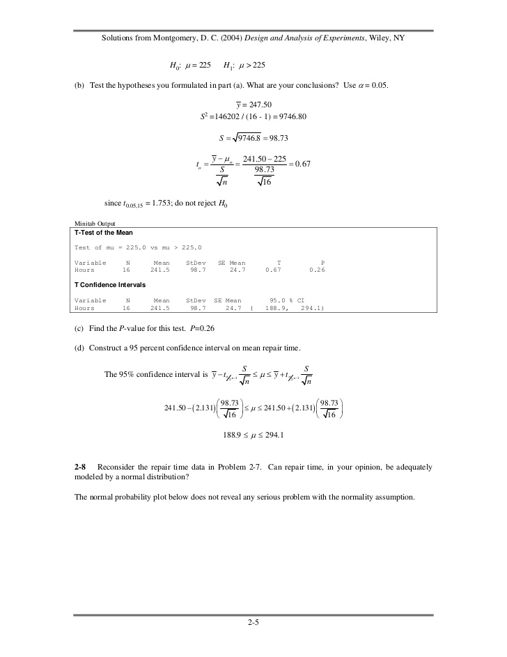
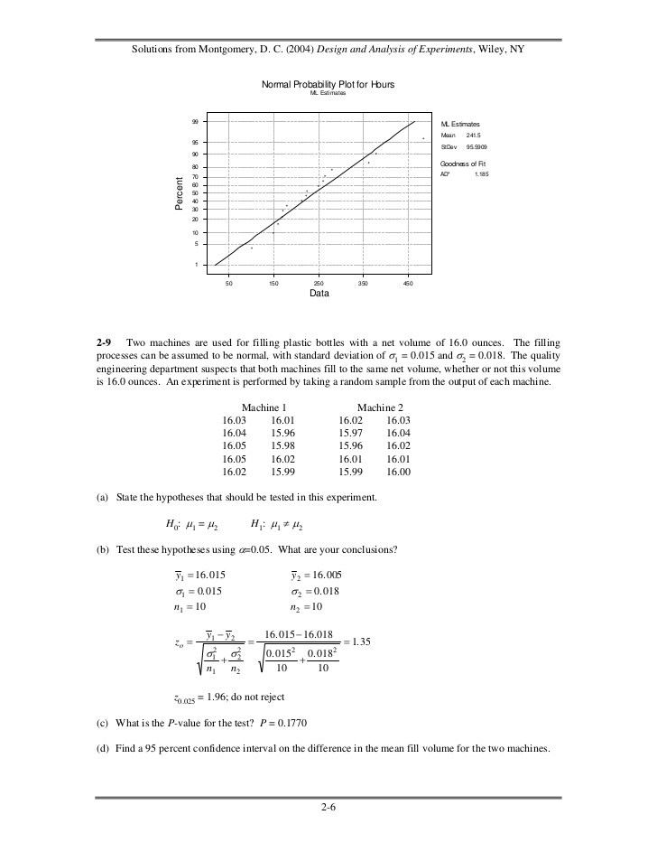
5. Solutions from Montgomery, D. C. (2004) Design and Analysis of Experiments, Wiley, NY H0: µ = 225 H1: µ > 225(b) Test the hypotheses you formulated in part (a). What are your conclusions? Use α = 0.05. y = 247.50 S2 =146202 / (16 - 1) = 9746.80 S = 9746.8 = 98.73 y − µo 241.50 − 225 to = = = 0.67 S 98.73 n 16 since t0.05,15 = 1.753; do not reject H0Minitab OutputT-Test of the MeanTest of mu = 225.0 vs mu > 225.0Variable N Mean StDev SE Mean T PHours 16 241.5 98.7 24.7 0.67 0.26T Confidence IntervalsVariable N Mean StDev SE Mean 95.0 % CIHours 16 241.5 98.7 24.7 ( 188.9, 294.1)(c) Find the P-value for this test. P=0.26(d) Construct a 95 percent confidence interval on mean repair time. S S The 95% confidence interval is y − tα 2,n−1 ≤ µ ≤ y + tα 2,n−1 n n ⎛ 98.73 ⎞ ⎛ 98.73 ⎞ 241.50 − ( 2.131) ⎜ ⎟ ≤ µ ≤ 241.50 + ( 2.131) ⎜ ⎟ ⎝ 16 ⎠ ⎝ 16 ⎠ 188.9 ≤ µ ≤ 294.12-8 Reconsider the repair time data in Problem 2-7. Can repair time, in your opinion, be adequatelymodeled by a normal distribution?The normal probability plot below does not reveal any serious problem with the normality assumption. 2-5

6. Solutions from Montgomery, D. C. (2004) Design and Analysis of Experiments, Wiley, NY Normal Probability Plot for Hours ML Estimates 99 ML Estimates Mean 241.5 95 StDev 95.5909 90 80 Goodness of Fit 70 AD* 1.185 Percent 60 50 40 30 20 10 5 1 50 150 250 350 450 Data2-9 Two machines are used for filling plastic bottles with a net volume of 16.0 ounces. The fillingprocesses can be assumed to be normal, with standard deviation of σ1 = 0.015 and σ2 = 0.018. The qualityengineering department suspects that both machines fill to the same net volume, whether or not this volumeis 16.0 ounces. An experiment is performed by taking a random sample from the output of each machine. Machine 1 Machine 2 16.03 16.01 16.02 16.03 16.04 15.96 15.97 16.04 16.05 15.98 15.96 16.02 16.05 16.02 16.01 16.01 16.02 15.99 15.99 16.00(a) State the hypotheses that should be tested in this experiment. H0: µ1 = µ2 H1: µ1 ≠ µ2(b) Test these hypotheses using α=0.05. What are your conclusions? y1 = 16. 015 y2 = 16. 005 σ 1 = 0. 015 σ 2 = 0. 018 n1 = 10 n2 = 10 y1 − y2 16. 015 − 16. 018 zo = = = 1. 35 σ1 2 σ2 0. 0152 0. 0182 + 2 + n1 n2 10 10 z0.025 = 1.96; do not reject(c) What is the P-value for the test? P = 0.1770(d) Find a 95 percent confidence interval on the difference in the mean fill volume for the two machines. 2-6

7. Solutions from Montgomery, D. C. (2004) Design and Analysis of Experiments, Wiley, NYThe 95% confidence interval is σ 12 σ2 2 σ 12 σ2 2 y1 − y 2 − z α 2 + ≤ µ 1 − µ 2 ≤ y1 − y 2 + z α 2 + n1 n2 n1 n2 2 2 0.015 0.018 0.015 2 0.018 2 (16.015 − 16.005) − (19.6) + ≤ µ1 − µ 2 ≤ (16.015 − 16.005) + (19.6) + 10 10 10 10 − 0.0045 ≤ µ 1 − µ 2 ≤ 0.02452-10 Two types of plastic are suitable for use by an electronic calculator manufacturer. The breakingstrength of this plastic is important. It is known that σ1 = σ2 = 1.0 psi. From random samples of n1 = 10and n2 = 12 we obtain y 1 = 162.5 and y 2 = 155.0. The company will not adopt plastic 1 unless itsbreaking strength exceeds that of plastic 2 by at least 10 psi. Based on the sample information, should theyuse plastic 1? In answering this questions, set up and test appropriate hypotheses using α = 0.01.Construct a 99 percent confidence interval on the true mean difference in breaking strength. H0: µ1 - µ2 =10 H1: µ1 - µ2 >10 y1 = 162.5 y2 = 155.0 σ1 = 1 σ2 = 1 n1 = 10 n2 = 10 y1 − y2 − 10 162. 5 − 155. 0 − 10 zo = = = −5.85 σ1 2 σ2 12 12 + 2 + n1 n2 10 12 z0.01 = 2.225; do not rejectThe 99 percent confidence interval is σ 12 σ2 2 σ 12 σ2 2 y1 − y 2 − z α 2 + ≤ µ 1 − µ 2 ≤ y1 − y 2 + z α 2 + n1 n2 n1 n2 12 12 12 12 (162.5 − 155.0) − (2.575) + ≤ µ1 − µ 2 ≤ (162.5 − 155.0) + (2.575) + 10 12 10 12 6.40 ≤ µ 1 − µ 2 ≤ 8.602-11 The following are the burning times (in minutes) of chemical flares of two different formulations.The design engineers are interested in both the means and variance of the burning times. Type 1 Type 2 65 82 64 56 81 67 71 69 57 59 83 74 66 75 59 82 82 70 65 79(a) Test the hypotheses that the two variances are equal. Use α = 0.05. 2-7

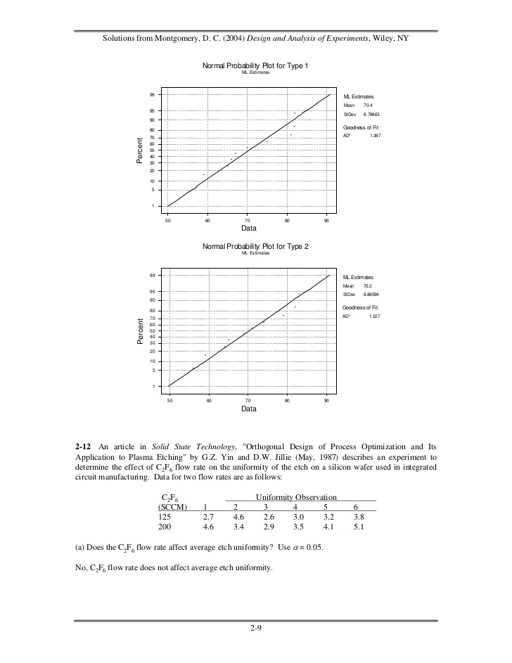
8. Solutions from Montgomery, D. C. (2004) Design and Analysis of Experiments, Wiley, NY H 0 : σ 12 = σ 2 2 S1 = 9.264 H1 : σ ≠ σ2 2 S 2 = 9.367 1 2 2 S1 8582 . F0 = 2 = = 0.98 S2 87.73 1 1 F0.025,9 ,9 = 4.03 F0.975,9 ,9 = = = 0.248 Do not reject. F0.025,9 ,9 4.03(b) Using the results of (a), test the hypotheses that the mean burning times are equal. Use α = 0.05. What is the P-value for this test? (n1 − 1) S1 + (n 2 − 1) S 2 156195 2 2 . Sp = 2 = = 86.775 n1 + n 2 − 2 18 S p = 9.32 y1 − y 2 70.4 − 70.2 t0 = = = 0.048 1 1 1 1 Sp + 9.32 + n1 n 2 10 10 t 0.025,18 = 2.101 Do not reject.From the computer output, t=0.05; do not reject. Also from the computer output P=0.96Minitab OutputTwo Sample T-Test and Confidence IntervalTwo sample T for Type 1 vs Type 2 N Mean StDev SE MeanType 1 10 70.40 9.26 2.9Type 2 10 70.20 9.37 3.095% CI for mu Type 1 - mu Type 2: ( -8.6, 9.0)T-Test mu Type 1 = mu Type 2 (vs not =): T = 0.05 P = 0.96 DF = 18Both use Pooled StDev = 9.32(c) Discuss the role of the normality assumption in this problem. Check the assumption of normality for both types of flares.The assumption of normality is required in the theoretical development of the t-test. However, moderatedeparture from normality has little impact on the performance of the t-test. The normality assumption ismore important for the test on the equality of the two variances. An indication of nonnormality would beof concern here. The normal probability plots shown below indicate that burning time for bothformulations follow the normal distribution. 2-8

9. Solutions from Montgomery, D. C. (2004) Design and Analysis of Experiments, Wiley, NY Normal Probability Plot for Type 1 ML Estimates 99 ML Estimates Mean 70.4 95 StDev 8.78863 90 80 Goodness of Fit 70 AD* 1.387 Percent 60 50 40 30 20 10 5 1 50 60 70 80 90 Data Normal Probability Plot for Type 2 ML Estimates 99 ML Estimates Mean 70.2 95 StDev 8.88594 90 80 Goodness of Fit 70 AD* 1.227 Percent 60 50 40 30 20 10 5 1 50 60 70 80 90 Data2-12 An article in Solid State Technology, "Orthogonal Design of Process Optimization and ItsApplication to Plasma Etching" by G.Z. Yin and D.W. Jillie (May, 1987) describes an experiment todetermine the effect of C2F6 flow rate on the uniformity of the etch on a silicon wafer used in integratedcircuit manufacturing. Data for two flow rates are as follows: C2F6 Uniformity Observation (SCCM) 1 2 3 4 5 6 125 2.7 4.6 2.6 3.0 3.2 3.8 200 4.6 3.4 2.9 3.5 4.1 5.1(a) Does the C2F6 flow rate affect average etch uniformity? Use α = 0.05.No, C2F6 flow rate does not affect average etch uniformity. 2-9

10. Solutions from Montgomery, D. C. (2004) Design and Analysis of Experiments, Wiley, NYMinitab OutputTwo Sample T-Test and Confidence IntervalTwo sample T for UniformityFlow Rat N Mean StDev SE Mean125 6 3.317 0.760 0.31200 6 3.933 0.821 0.3495% CI for mu (125) - mu (200): ( -1.63, 0.40)T-Test mu (125) = mu (200) (vs not =): T = -1.35 P = 0.21 DF = 10Both use Pooled StDev = 0.791(b) What is the P-value for the test in part (a)? From the computer printout, P=0.21(c) Does the C2F6 flow rate affect the wafer-to-wafer variability in etch uniformity? Use α = 0.05. H 0 : σ 12 = σ 2 2 H1 : σ 12 ≠ σ 2 2 F0.05,5,5 = 5.05 0.5776 F0 = = 0.86 0.6724Do not reject; C2F6 flow rate does not affect wafer-to-wafer variability.(d) Draw box plots to assist in the interpretation of the data from this experiment.The box plots shown below indicate that there is little difference in uniformity at the two gas flow rates.Any observed difference is not statistically significant. See the t-test in part (a). 5 Uniformity 4 3 125 200 Flow Rate2-13 A new filtering device is installed in a chemical unit. Before its installation, a random sample 2yielded the following information about the percentage of impurity: y 1 = 12.5, S1 =101.17, and n1 = 8. 2After installation, a random sample yielded y 2 = 10.2, S2 = 94.73, n2 = 9.(a) Can you concluded that the two variances are equal? Use α = 0.05. 2-10

11. Solutions from Montgomery, D. C. (2004) Design and Analysis of Experiments, Wiley, NY H 0 : σ1 = σ 2 2 2 H1 : σ 1 ≠ σ 2 2 2 F0.025 ,7 ,8 = 4.53 S12 101.17 F0 = 2 = = 1.07 S2 94.73Do Not Reject. Assume that the variances are equal.(b) Has the filtering device reduced the percentage of impurity significantly? Use α = 0.05. H 0 : µ1 = µ 2 H1 : µ1 ≠ µ 2 ( n1 − 1 )S12 + ( n2 − 1 )S 2 ( 8 − 1 )( 101.17 ) + ( 9 − 1 )( 94.73 ) 2 Sp = 2 = = 97.74 n1 + n2 − 2 8+9−2 S p = 9.89 y1 − y2 12.5 − 10.2 t0 = = = 0.479 1 1 1 1 Sp + 9.89 + n1 n2 8 9 t0.05 ,15 = 1.753Do not reject. There is no evidence to indicate that the new filtering device has affected the mean2-14 Photoresist is a light-sensitive material applied to semiconductor wafers so that the circuit patterncan be imaged on to the wafer. After application, the coated wafers are baked to remove the solvent in thephotoresist mixture and to harden the resist. Here are measurements of photoresist thickness (in kÅ) foreight wafers baked at two different temperatures. Assume that all of the runs were made in random order. 95 ºC 100 ºC 11.176 5.263 7.089 6.748 8.097 7.461 11.739 7.015 11.291 8.133 10.759 7.418 6.467 3.772 8.315 8.963(a) Is there evidence to support the claim that the higher baking temperature results in wafers with a lower mean photoresist thickness? Use α = 0.05. 2-11

12. Solutions from Montgomery, D. C. (2004) Design and Analysis of Experiments, Wiley, NY H 0 : µ1 = µ2 H1 : µ1 ≠ µ2 (n1 − 1) S12 + (n2 − 1) S22 (8 − 1)(4.41) + (8 − 1)(2.54) Sp = 2 = = 3.48 n1 + n2 − 2 8+8−2 S p = 1.86 y1 − y2 9.37 − 6.89 t0 = = = 2.65 1 1 1 1 Sp + 1.86 + n1 n2 8 8 t0.05,14 = 1.761Since t0.05,14 = 1.761, reject H0. There appears to be a lower mean thickness at the higher temperature. Thisis also seen in the computer output.Minitab OutputTwo-Sample T-Test and CI: Thickness, TempTwo-sample T for ThicknessTemp N Mean StDev SE Mean 95 8 9.37 2.10 0.74100 8 6.89 1.60 0.56Difference = mu ( 95) - mu (100)Estimate for difference: 2.47595% CI for difference: (0.476, 4.474)T-Test of difference = 0 (vs not =): T-Value = 2.65 P-Value = 0.019 DF = 14Both use Pooled StDev = 1.86(b) What is the P-value for the test conducted in part (a)? P = 0.019(c) Find a 95% confidence interval on the difference in means. Provide a practical interpretation of this interval.From the computer output the 95% confidence interval is 0.476 ≤ µ1 − µ 2 ≤ 4.474 . This confidence intervaldoesnot include 0 in it, there for there is a difference in the two temperatures on the thickness of the photoresist.(d) Draw dot diagrams to assist in interpreting the results from this experiment. 2-12

13. Solutions from Montgomery, D. C. (2004) Design and Analysis of Experiments, Wiley, NY Dotplot of Thickness vs Temp Temp 95 3.6 4.8 6.0 7.2 8.4 9.6 10.8 12.0 100 Thickness(e) Check the assumption of normality of the photoresist thickness. Normal Probability Plot for Thick@95 ML Estimates - 95% CI 99 ML Estimates Mean 9.36663 95 StDev 1.96396 90 80 Goodness of Fit 70 AD* 1.767 Percent 60 50 40 30 20 10 5 1 5 10 15 Data 2-13

14. Solutions from Montgomery, D. C. (2004) Design and Analysis of Experiments, Wiley, NY Normal Probability Plot for Thick@100 ML Estimates - 95% CI 99 ML Estimates Mean 6.89163 95 StDev 1.49207 90 80 Goodness of Fit 70 AD* 1.567 Percent 60 50 40 30 20 10 5 1 2 7 12 DataThere are no significant deviations from the normality assumptions.(f) Find the power of this test for detecting an actual difference in means of 2.5 kÅ.Minitab OutputPower and Sample Size2-Sample t TestTesting mean 1 = mean 2 (versus not =)Calculating power for mean 1 = mean 2 + differenceAlpha = 0.05 Sigma = 1.86 SampleDifference Size Power 2.5 8 0.7056(g) What sample size would be necessary to detect an actual difference in means of 1.5 kÅ with a power of at least 0.9?.Minitab OutputPower and Sample Size2-Sample t TestTesting mean 1 = mean 2 (versus not =)Calculating power for mean 1 = mean 2 + differenceAlpha = 0.05 Sigma = 1.86 Sample Target ActualDifference Size Power Power 1.5 34 0.9000 0.9060 2-14

15. Solutions from Montgomery, D. C. (2004) Design and Analysis of Experiments, Wiley, NYThis result makes intuitive sense. More samples are needed to detect a smaller difference.2-15 Front housings for cell phones are manufactured in an injection molding process. The time the partis allowed to cool in the mold before removal is thought to influence the occurrence of a particularlytroublesome cosmetic defect, flow lines, in the finished housing. After manufacturing, the housings areinspected visually and assigned a score between 1 and 10 based on their appearance, with 10 correspondingto a perfect part and 1 corresponding to a completely defective part. An experiment was conducted usingtwo cool-down times, 10 seconds and 20 seconds, and 20 housings were evaluated at each level of cool-down time. The data are shown below. 10 Seconds 20 Seconds 1 3 7 6 2 6 8 9 1 5 5 5 3 3 9 7 5 2 5 4 1 1 8 6 5 6 6 8 2 8 4 5 3 2 6 8 5 3 7 7(a) Is there evidence to support the claim that the longer cool-down time results in fewer appearance defects? Use α = 0.05.Minitab OutputTwo-Sample T-Test and CI: 10 seconds, 20 secondsTwo-sample T for 10 seconds vs 20 seconds N Mean StDev SE Mean10 secon 20 3.35 2.01 0.4520 secon 20 6.50 1.54 0.34Difference = mu 10 seconds - mu 20 secondsEstimate for difference: -3.15095% CI for difference: (-4.295, -2.005)T-Test of difference = 0 (vs not =): T-Value = -5.57 P-Value = 0.000 DF = 38Both use Pooled StDev = 1.79(b) What is the P-value for the test conducted in part (a)? From the Minitab output, P = 0.000(c) Find a 95% confidence interval on the difference in means. Provide a practical interpretation of this interval.From the computer output, −4.295 ≤ µ1 − µ 2 ≤ −2.005 . This interval does not contain 0. The two samples aredifferent. The 20 second cooling time gives a cosmetically better housing.(d) Draw dot diagrams to assist in interpreting the results from this experiment. 2-15

16. Solutions from Montgomery, D. C. (2004) Design and Analysis of Experiments, Wiley, NY Dotplot of Ranking vs C4 C4 10 sec 20 sec 2 4 6 8 Ranking(e) Check the assumption of normality for the data from this experiment. Normal Probability Plot for 10 seconds ML Estimates - 95% CI 99 ML Estimates Mean 3.35 95 StDev 1.95640 90 80 Goodness of Fit 70 AD* 1.252 Percent 60 50 40 30 20 10 5 1 0 4 8 Data 2-16

17. Solutions from Montgomery, D. C. (2004) Design and Analysis of Experiments, Wiley, NY Normal Probability Plot for 20 seconds ML Estimates - 95% CI 99 ML Estimates Mean 6.5 95 StDev 1.50000 90 80 Goodness of Fit 70 AD* 0.988 Percent 60 50 40 30 20 10 5 1 2 3 4 5 6 7 8 9 10 11 DataThere are no significant departures from normality.2-16 Twenty observations on etch uniformity on silicon wafers are taken during a qualificationexperiment for a plasma etcher. The data are as follows: 5.34 6.65 4.76 5.98 7.25 6.00 7.55 5.54 5.62 6.21 5.97 7.35 5.44 4.39 4.98 5.25 6.35 4.61 6.00 5.32(a) Construct a 95 percent confidence interval estimate of σ2. ( n − 1) S 2 ≤ σ 2 ≤ ( n − 1) S 2 χα 2 , n −1 2 χ (1−α ), n −1 2 2 ( 20 − 1)( 0.88907 ) ( 20 − 1)( 0.88907 ) 2 2 ≤σ2 ≤ 32.852 8.907 0.457 ≤ σ 2 ≤ 1.686(b) Test the hypothesis that σ2 = 1.0. Use α = 0.05. What are your conclusions? H0 :σ 2 = 1 H1 : σ 2 ≠ 1 SS χ0 = 2 = 15.019 σ0 2 2-17

18. Solutions from Montgomery, D. C. (2004) Design and Analysis of Experiments, Wiley, NY χ 0.025,19 = 32.852 2 χ 0.975,19 = 8.907 2Do not reject. There is no evidence to indicate that σ 2 ≠ 1(c) Discuss the normality assumption and its role in this problem.The normality assumption is much more important when analyzing variances then when analyzing means.A moderate departure from normality could cause problems with both statistical tests and confidenceintervals. Specifically, it will cause the reported significance levels to be incorrect.(d) Check normality by constructing a normal probability plot. What are your conclusions?The normal probability plot indicates that there is not any serious problem with the normality assumption. Normal Probability Plot for Uniformity ML Estimates 99 ML Estimates Mean 5.828 95 StDev 0.866560 90 80 Goodness of Fit 70 AD* 0.835 Percent 60 50 40 30 20 10 5 1 3.8 4.8 5.8 6.8 7.8 Data2-17 The diameter of a ball bearing was measured by 12 inspectors, each using two different kinds ofcalipers. The results were: Inspector Caliper 1 Caliper 2 Difference Difference^2 1 0.265 0.264 .001 .000001 2 0.265 0.265 .000 0 3 0.266 0.264 .002 .000004 4 0.267 0.266 .001 .000001 5 0.267 0.267 .000 0 6 0.265 0.268 -.003 .000009 7 0.267 0.264 .003 .000009 8 0.267 0.265 .002 .000004 9 0.265 0.265 .000 0 10 0.268 0.267 .001 .000001 11 0.268 0.268 .000 0 12 0.265 0.269 -.004 .000016 ∑ = 0.003 ∑ = 0.000045 2-18

19. Solutions from Montgomery, D. C. (2004) Design and Analysis of Experiments, Wiley, NY(a) Is there a significant difference between the means of the population of measurements represented by the two samples? Use α = 0.05. H 0 : µ1 = µ 2 H0 : µd = 0 or equivalently H1 : µ 1 ≠ µ 2 H1 : µ d ≠ 0Minitab OutputPaired T-Test and Confidence IntervalPaired T for Caliper 1 - Caliper 2 N Mean StDev SE MeanCaliper 12 0.266250 0.001215 0.000351Caliper 12 0.266000 0.001758 0.000508Difference 12 0.000250 0.002006 0.00057995% CI for mean difference: (-0.001024, 0.001524)T-Test of mean difference = 0 (vs not = 0): T-Value = 0.43 P-Value = 0.674(b) Find the P-value for the test in part (a). P=0.674(c) Construct a 95 percent confidence interval on the difference in the mean diameter measurements for the two types of calipers. Sd S d − tα ≤ µ D ( = µ1 − µ 2 ) ≤ d + tα ,n −1 d , n −1 2 n 2 n 0.002 0.002 0.00025 − 2.201 ≤ µ d ≤ 0.00025 + 2.201 12 12 −0.00102 ≤ µ d ≤ 0.001522-18 An article in the Journal of Strain Analysis (vol.18, no. 2, 1983) compares several procedures forpredicting the shear strength for steel plate girders. Data for nine girders in the form of the ratio ofpredicted to observed load for two of these procedures, the Karlsruhe and Lehigh methods, are as follows: Girder Karlsruhe Method Lehigh Method Difference Difference^2 S1/1 1.186 1.061 0.125 0.015625 S2/1 1.151 0.992 0.159 0.025281 S3/1 1.322 1.063 0.259 0.067081 S4/1 1.339 1.062 0.277 0.076729 S5/1 1.200 1.065 0.135 0.018225 S2/1 1.402 1.178 0.224 0.050176 S2/2 1.365 1.037 0.328 0.107584 S2/3 1.537 1.086 0.451 0.203401 S2/4 1.559 1.052 0.507 0.257049 Sum = 2.465 0.821151 Average = 0.274(a) Is there any evidence to support a claim that there is a difference in mean performance between the two methods? Use α = 0.05. H 0 : µ1 = µ 2 H0 : µd = 0 or equivalently H1 : µ 1 ≠ µ 2 H1 : µ d ≠ 0 2-19

20. Solutions from Montgomery, D. C. (2004) Design and Analysis of Experiments, Wiley, NY 1 n 1 d= ∑ di = 9 ( 2.465) = 0.274 n i =1 1 ⎡ n 2 1 ⎛ n ⎞2 ⎤ 2 1 ⎢ ∑ di − ⎜ ∑ di ⎟ ⎥ ⎡ 2⎤ 2 1 ⎢ 0.821151 − (2.465) ⎥ n ⎝ i =1 ⎠ ⎥ sd = ⎢ i =1 =⎢ 9 ⎥ = 0.135 ⎢ n −1 ⎥ 9 −1 ⎢ ⎥ ⎢ ⎥ ⎢ ⎥ ⎣ ⎦ ⎣ ⎦ d 0.274 t0 = = = 6.08 Sd 0.135 n 9 t α 2 ,n −1 = t 0.025 ,9 = 2.306 , reject the null hypothesis.Minitab OutputPaired T-Test and Confidence IntervalPaired T for Karlsruhe - Lehigh N Mean StDev SE MeanKarlsruh 9 1.3401 0.1460 0.0487Lehigh 9 1.0662 0.0494 0.0165Difference 9 0.2739 0.1351 0.045095% CI for mean difference: (0.1700, 0.3777)T-Test of mean difference = 0 (vs not = 0): T-Value = 6.08 P-Value = 0.000(b) What is the P-value for the test in part (a)? P=0.0002(c) Construct a 95 percent confidence interval for the difference in mean predicted to observed load. Sd Sd d − tα ,n −1 ≤ µ d ≤ d + tα ,n −1 2 n n 2 0.135 0.135 0.274 − 2.306 ≤ µ d ≤ 0.274 + 2.306 9 9 0.17023 ≤ µ d ≤ 0.37777(d) Investigate the normality assumption for both samples. Normal Probability Plot .999 .99 .95 Probability .80 .50 .20 .05 .01 .001 1.15 1.25 1.35 1.45 1.55 Karlsruhe Av erage: 1.34011 Anderson-Darling Normality Test StDev : 0.146031 A-Squared: 0.286 N: 9 P-Value: 0.537 2-20

21. Solutions from Montgomery, D. C. (2004) Design and Analysis of Experiments, Wiley, NY Normal Probability Plot .999 .99 .95 Probability .80 .50 .20 .05 .01 .001 1.00 1.05 1.10 1.15 Lehigh Av erage: 1.06622 Anderson-Darling Normality Test StDev : 0.0493806 A-Squared: 0.772 N: 9 P-Value: 0.028(e) Investigate the normality assumption for the difference in ratios for the two methods. Normal Probability Plot .999 .99 .95 Probability .80 .50 .20 .05 .01 .001 0.12 0.22 0.32 0.42 0.52 Difference Av erage: 0.273889 Anderson-Darling Normality Test StDev : 0.135099 A-Squared: 0.318 N: 9 P-Value: 0.464(f) Discuss the role of the normality assumption in the paired t-test.As in any t-test, the assumption of normality is of only moderate importance. In the paired t-test, theassumption of normality applies to the distribution of the differences. That is, the individual samplemeasurements do not have to be normally distributed, only their difference.2-19 The deflection temperature under load for two different formulations of ABS plastic pipe is beingstudied. Two samples of 12 observations each are prepared using each formulation, and the deflectiontemperatures (in °F) are reported below: Formulation 1 Formulation 2 212 199 198 177 176 198 194 213 216 197 185 188 211 191 200 206 200 189 193 195 184 201 197 203 2-21

22. Solutions from Montgomery, D. C. (2004) Design and Analysis of Experiments, Wiley, NY(a) Construct normal probability plots for both samples. Do these plots support assumptions of normality and equal variance for both samples? Normal Probability Plot .999 .99 .95 Probability .80 .50 .20 .05 .01 .001 185 195 205 215 Form 1 Av erage: 200.5 Anderson-Darling Normality Test StDev : 10.1757 A-Squared: 0.450 N: 12 P-Value: 0.227 Normal Probability Plot .999 .99 .95 Probability .80 .50 .20 .05 .01 .001 175 185 195 205 Form 2 Av erage: 193.083 Anderson-Darling Normality Test StDev : 9.94949 A-Squared: 0.443 N: 12 P-Value: 0.236(b) Do the data support the claim that the mean deflection temperature under load for formulation 1 exceeds that of formulation 2? Use α = 0.05.Minitab OutputTwo Sample T-Test and Confidence IntervalTwo sample T for Form 1 vs Form 2 N Mean StDev SE MeanForm 1 12 200.5 10.2 2.9Form 2 12 193.08 9.95 2.995% CI for mu Form 1 - mu Form 2: ( -1.1, 15.9)T-Test mu Form 1 = mu Form 2 (vs >): T = 1.81 P = 0.042 DF = 22Both use Pooled StDev = 10.1(c) What is the P-value for the test in part (a)? P = 0.042 2-22

23. Solutions from Montgomery, D. C. (2004) Design and Analysis of Experiments, Wiley, NY2-20 Refer to the data in problem 2-19. Do the data support a claim that the mean deflection temperatureunder load for formulation 1 exceeds that of formulation 2 by at least 3 °F?Yes, formulation 1 exceeds formulation 2 by at least 3 °F.Minitab OutputTwo-Sample T-Test and CI: Form1, Form2Two-sample T for Form1 vs Form2 N Mean StDev SE MeanForm1 12 200.5 10.2 2.9Form2 12 193.08 9.95 2.9rDifference = mu Form1 - mu Form2Estimate for difference: 7.4295% lower bound for difference: 0.36T-Test of difference = 3 (vs >): T-Value = 1.08 P-Value = 0.147 DF = 22Both use Pooled StDev = 10.12-21 In semiconductor manufacturing, wet chemical etching is often used to remove silicon from thebacks of wafers prior to metalization. The etch rate is an important characteristic of this process. Twodifferent etching solutionsare being evaluated. Eight randomly selected wafers have been etched in eachsolution and the observed etch rates (in mils/min) are shown below: Solution 1 Solution 2 9.9 10.6 10.2 10.6 9.4 10.3 10.0 10.2 10.0 9.3 10.7 10.4 10.3 9.8 10.5 10.3(a) Do the data indicate that the claim that both solutions have the same mean etch rate is valid? Use α = 0.05 and assume equal variances.See the Minitab output below.Minitab OutputTwo Sample T-Test and Confidence IntervalTwo sample T for Solution 1 vs Solution 2 N Mean StDev SE MeanSolution 8 9.925 0.465 0.16Solution 8 10.362 0.233 0.08295% CI for mu Solution - mu Solution: ( -0.83, -0.043)T-Test mu Solution = mu Solution (vs not =):T = -2.38 P = 0.032 DF = 14Both use Pooled StDev = 0.368(b) Find a 95% confidence interval on the difference in mean etch rate.From the Minitab output, -0.83 to –0.043.(c) Use normal probability plots to investigate the adequacy of the assumptions of normality and equal variances. 2-23

24. Solutions from Montgomery, D. C. (2004) Design and Analysis of Experiments, Wiley, NY Normal Probability Plot .999 .99 .95 Probability .80 .50 .20 .05 .01 .001 9.5 10.0 10.5 Solution 1 Av erage: 9.925 Anderson-Darling Normality Test StDev : 0.465219 A-Squared: 0.222 N: 8 P-Value: 0.743 Normal Probability Plot .999 .99 .95 Probability .80 .50 .20 .05 .01 .001 10.0 10.1 10.2 10.3 10.4 10.5 10.6 10.7 Solution 2 Av erage: 10.3625 Anderson-Darling Normality Test StDev : 0.232609 A-Squared: 0.158 N: 8 P-Value: 0.919Both the normality and equality of variance assumptions are valid.2-22 Two popular pain medications are being compared on the basis of the speed of absorption by thebody. Specifically, tablet 1 is claimed to be absorbed twice as fast as tablet 2. Assume that σ 12 and σ 2 2are known. Develop a test statistic for H0: 2µ1 = µ2 H1: 2µ1 ≠ µ2 ⎛ 4σ 2 σ 2 ⎞ 2 y1 − y2 ~ N ⎜ 2 µ1 − µ 2 , 1 + 2 ⎟ , assuming that the data is normally distributed. ⎝ n1 n2 ⎠ 2 y1 − y2 The test statistic is: zo = , reject if zo > zα 2 4 σ1 σ 2 2 + 2 n1 n22-23 Suppose we are testing H0: µ1 = µ2 H1: µ1 ≠ µ2 2-24

25. Solutions from Montgomery, D. C. (2004) Design and Analysis of Experiments, Wiley, NYwhere σ 12 and σ 2 are known. Our sampling resources are constrained such that n1 + n2 = N. How should 2we allocate the N observations between the two populations to obtain the most powerful test? The most powerful test is attained by the n1 and n2 that maximize zo for given y1 − y2 . Thus, we chose n1 and n2 to y1 − y 2 , subject to n1 + n2 = N. max zo = 2 2 σ1 σ2 + n1 n2 σ1 2 σ2 σ1 2 σ2 This is equivalent to min L = + 2 = + 2 , subject to n1 + n2 = N. n1 n2 n1 N − n1 Now dL = −σ 1 + σ 2 2 2 = 0 , implies that n1 / n2 = σ1 / σ2. ( N − n1 ) 2 2 dn1 n1 Thus n1 and n2 are assigned proportionally to the ratio of the standard deviations. This has intuitive appeal, as it allocates more observations to the population with the greatest variability.2-24 Develop Equation 2-46 for a 100(1 - α) percent confidence interval for the variance of a normaldistribution. SS ~ χ n −1 . Thus, P ⎧ χ 2 ⎨ 2 ≤ SS ⎫ ≤ χ α2 ,n−1 ⎬ = 1 − α . Therefore, σ α σ2 2 ⎩ ⎭ 1− ,n−1 2 2 ⎧ ⎫ ⎪ SS SS ⎪ , P ⎨ 2 ≤ σ 2 ≤ 2 ⎬ = 1−α χ α ,n−1 ⎪ 2 χ1−α ,n−1 ⎪ ⎩ 2 ⎭ ⎡ ⎤ so ⎢ SS , SS ⎥ is the 100(1 - α)% confidence interval on σ2. ⎢ χ α2 ,n−1 χ12−α ,n−1 ⎥ ⎣ 2 2 ⎦2-25 Develop Equation 2-50 for a 100(1 - α) percent confidence interval for the ratio σ 1 / σ 2 , where σ 1 2 2 2and σ 2 are the variances of two normal distributions. 2 S2 σ 2 2 2 ~ Fn2 −1,n1 −1 S12 σ 12 ⎧ S2 σ 2 ⎫ P ⎨ F1−α 2 ,n2 −1,n1 −1 ≤ 2 2 ≤ Fα ⎬ = 1 − α or ⎩ S1 σ 1 2 2 ,n −1,n1−1 2 2 ⎭ ⎧S 2 σ 2 S 2 ⎫ P ⎨ 12 F1−α 2 ,n2 −1,n1 −1 ≤ 12 ≤ 12 Fα ⎬ = 1−α ⎩ S2 σ 2 S2 2 ,n2 −1,n1−1 ⎭2-26 Develop an equation for finding a 100(1 - α) percent confidence interval on the difference in themeans of two normal distributions where σ 12 ≠ σ 2 . Apply your equation to the portland cement 2experiment data, and find a 95% confidence interval. 2-25

26. Solutions from Montgomery, D. C. (2004) Design and Analysis of Experiments, Wiley, NY ( y1 − y2 ) − ( µ1 − µ2 ) ~ t 2 ,υ α S12 S 2 2 + n1 n2 S12 S2 2 S2 S2 tα 2 ,υ + ≤ ( y1 − y2 ) − ( µ1 − µ 2 ) ≤ tα 2 ,υ 1 + 2 n1 n2 n1 n2 S12 S 2 2 S2 S2 ( y1 − y2 ) − t α 2 ,υ + ≤ ( µ1 − µ 2 ) ≤ ( y1 − y2 ) + tα 2,υ 1 + 2 n1 n2 n1 n2 2 ⎛ S12 S 2 ⎞ 2 ⎜ + ⎟ υ = ⎝ 12 2 ⎠ 2 where n n ⎛ S12 ⎞ ⎛ S 2 ⎞ 2 ⎜ ⎟ ⎜ ⎟ ⎝ n1 ⎠ + ⎝ n2 ⎠ n1 − 1 n2 − 1 Using the data from Table 2-1 n1 = 10 n 2 = 10 y1 = 16.764 y 2 = 17.343 2 S1 = 0100138 . S 2 = 0.0614622 2 0.100138 0.0614622 (16.764 − 17.343) − 2.110 + ≤ ( µ1 − µ 2 ) ≤ 10 10 0.100138 0.0614622 (16.764 − 17.343) + 2.110 + 10 10 2 ⎛ 0.100138 0.0614622 ⎞ ⎜ + ⎟ ⎝ 10 10 ⎠ where υ = 2 2 = 17.024 ≅ 17 ⎛ 0.100138 ⎞ ⎛ 0.0614622 ⎞ ⎜ ⎟ ⎜ ⎟ ⎝ 10 ⎠ ⎝ 10 ⎠ + 10 − 1 10 − 1 −1.426 ≤ ( µ1 − µ2 ) ≤ −0.889This agrees with the result in Table 2-2.2-27 Construct a data set for which the paired t-test statistic is very large, but for which the usual two-sample or pooled t-test statistic is small. In general, describe how you created the data. Does this give youany insight regarding how the paired t-test works? A B delta 7.1662 8.2416 1.07541 2.3590 2.4555 0.09650 19.9977 21.1018 1.10412 0.9077 2.3401 1.43239 -15.9034 -15.0013 0.90204 -6.0722 -5.5941 0.47808 2-26

27. Solutions from Montgomery, D. C. (2004) Design and Analysis of Experiments, Wiley, NY 9.9501 10.6910 0.74085 -1.0944 -0.1358 0.95854 -4.6907 -3.3446 1.34615 -6.6929 -5.9303 0.76256Minitab OutputPaired T-Test and Confidence IntervalPaired T for A - B N Mean StDev SE MeanA 10 0.59 10.06 3.18B 10 1.48 10.11 3.20Difference 10 -0.890 0.398 0.12695% CI for mean difference: (-1.174, -0.605)T-Test of mean difference = 0 (vs not = 0): T-Value = -7.07 P-Value = 0.000Two Sample T-Test and Confidence IntervalTwo sample T for A vs B N Mean StDev SE MeanA 10 0.6 10.1 3.2B 10 1.5 10.1 3.295% CI for mu A - mu B: ( -10.4, 8.6)T-Test mu A = mu B (vs not =): T = -0.20 P = 0.85 DF = 18Both use Pooled StDev = 10.1These two sets of data were created by making the observation for A and B moderately different withineach pair (or block), but making the observations between pairs very different. The fact that the differencebetween pairs is large makes the pooled estimate of the standard deviation large and the two-sample t-teststatistic small. Therefore the fairly small difference between the means of the two treatments that is presentwhen they are applied to the same experimental unit cannot be detected. Generally, if the blocks are verydifferent, then this will occur. Blocking eliminates the variabiliy associated with the nuisance variable thatthey represent.2-28 Consider the experiment described in problem 2-11. If the mean burning times of the two flamesdiffer by as much as 2 minutes, find the power of the test. What sample size would be required to detect anactual difference in mean burning time of 1 minute with a power of at least 0.90?Minitab OutputPower and Sample Size2-Sample t TestTesting mean 1 = mean 2 (versus not =)Calculating power for mean 1 = mean 2 + differenceAlpha = 0.05 Sigma = 9.32 Sample Target ActualDifference Size Power Power 2 458 0.9000 0.90042-29 Reconsider the bottle filling experiment described in Problem 2-9. Rework this problem assumingthat the two population variances are unknown but equal. 2-27

28. Solutions from Montgomery, D. C. (2004) Design and Analysis of Experiments, Wiley, NYMinitab OutputTwo-Sample T-Test and CI: Machine 1, Machine 2Two-sample T for Machine 1 vs Machine 2 N Mean StDev SE MeanMachine 10 16.0150 0.0303 0.0096Machine 10 16.0050 0.0255 0.0081Difference = mu Machine 1 - mu Machine 2Estimate for difference: 0.010095% CI for difference: (-0.0163, 0.0363)T-Test of difference = 0 (vs not =): T-Value = 0.80 P-Value = 0.435 DF = 18Both use Pooled StDev = 0.0280The hypothesis test is the same: H0: µ1 = µ2 H1: µ1 ≠ µ2The conclusions are the same as Problem 2-9, do not reject H0. There is no difference in the machines.The P-value for this anlysis is 0.435.The confidence interval is (-0.0163, 0.0363). This interval contains 0. There is no difference in machines.2-29 Consider the data from problem 2-9. If the mean fill volume of the two machines differ by as muchas 0.25 ounces, what is the power of the test used in problem 2-9? What sample size could result in apower of at least 0.9 if the actual difference in mean fill volume is 0.25 ounces?Minitab OutputPower and Sample Size2-Sample t TestTesting mean 1 = mean 2 (versus not =)Calculating power for mean 1 = mean 2 + differenceAlpha = 0.05 Sigma = 0.028 SampleDifference Size Power 0.25 10 1.0000Minitab OutputPower and Sample Size2-Sample t TestTesting mean 1 = mean 2 (versus not =)Calculating power for mean 1 = mean 2 + differenceAlpha = 0.05 Sigma = 0.028 Sample Target ActualDifference Size Power Power 0.25 2 0.9000 0.9805 2-28

29. Solutions from Montgomery, D. C. (2004) Design and Analysis of Experiments, Wiley, NY Chapter 3 Experiments with a Single Factor: The Analysis of Variance Solutions3-1 The tensile strength of portland cement is being studied. Four different mixing techniques can beused economically. The following data have been collected: Mixing Technique Tensile Strength (lb/in2) 1 3129 3000 2865 2890 2 3200 3300 2975 3150 3 2800 2900 2985 3050 4 2600 2700 2600 2765(a) Test the hypothesis that mixing techniques affect the strength of the cement. Use α = 0.05.Design Expert OutputResponse: Tensile Strengthin lb/in^2 ANOVA for Selected Factorial Model Analysis of variance table [Partial sum of squares] Sum of Mean F Source Squares DF Square Value Prob > F Model 4.897E+005 3 1.632E+005 12.73 0.0005 significant A 4.897E+005 3 1.632E+005 12.73 0.0005 Residual 1.539E+005 12 12825.69 Lack of Fit 0.000 0 Pure Error 1.539E+005 12 12825.69 Cor Total 6.436E+005 15 The Model F-value of 12.73 implies the model is significant. There is only a 0.05% chance that a "Model F-Value" this large could occur due to noise. Treatment Means (Adjusted, If Necessary) Estimated Standard Mean Error 1-1 2971.00 56.63 2-2 3156.25 56.63 3-3 2933.75 56.63 4-4 2666.25 56.63 Mean Standard t for H0 Treatment Difference DF Error Coeff=0 Prob > |t| 1 vs 2 -185.25 1 80.08 -2.31 0.0392 1 vs 3 37.25 1 80.08 0.47 0.6501 1 vs 4 304.75 1 80.08 3.81 0.0025 2 vs 3 222.50 1 80.08 2.78 0.0167 2 vs 4 490.00 1 80.08 6.12 < 0.0001 3 vs 4 267.50 1 80.08 3.34 0.0059The F-value is 12.73 with a corresponding P-value of .0005. Mixing technique has an effect.(b) Construct a graphical display as described in Section 3-5.3 to compare the mean tensile strengths for the four mixing techniques. What are your conclusions? MS E 12825.7 S yi . = = = 56.625 n 4 3-1

30. Solutions from Montgomery, D. C. (2004) Design and Analysis of Experiments, Wiley, NY S c a le d t D is t r ib u t io n (4 ) (3 ) (1 ) (2 ) 2700 2800 2900 3000 3100 T e n s ile S t r e n g t hBased on examination of the plot, we would conclude that µ1 and µ3 are the same; that µ 4 differs fromµ1 and µ3 , that µ 2 differs from µ1 and µ3 , and that µ 2 and µ 4 are different.(c) Use the Fisher LSD method with α=0.05 to make comparisons between pairs of means. 2MS E LSD = t α ,N − a n 2 2( 12825.7 ) LSD = t 0.025 ,16 − 4 4 LSD = 2.179 6412.85 = 174.495 Treatment 2 vs. Treatment 4 = 3156.250 - 2666.250 = 490.000 > 174.495 Treatment 2 vs. Treatment 3 = 3156.250 - 2933.750 = 222.500 > 174.495 Treatment 2 vs. Treatment 1 = 3156.250 - 2971.000 = 185.250 > 174.495 Treatment 1 vs. Treatment 4 = 2971.000 - 2666.250 = 304.750 > 174.495 Treatment 1 vs. Treatment 3 = 2971.000 - 2933.750 = 37.250 < 174.495 Treatment 3 vs. Treatment 4 = 2933.750 - 2666.250 = 267.500 > 174.495The Fisher LSD method is also presented in the Design-Expert computer output above. The results agreewith the graphical method for this experiment.(d) Construct a normal probability plot of the residuals. What conclusion would you draw about the validity of the normality assumption?There is nothing unusual about the normal probability plot of residuals. 3-2

31. Solutions from Montgomery, D. C. (2004) Design and Analysis of Experiments, Wiley, NY Normal plot of residuals 99 95 N orm al % probability 90 80 70 50 30 20 10 5 1 -1 8 1 .2 5 -9 6 .4 3 7 5 -1 1 .6 2 5 7 3 .1 8 7 5 158 R es idual(e) Plot the residuals versus the predicted tensile strength. Comment on the plot.There is nothing unusual about this plot. Residuals vs. Predicted 158 73.1875 Res iduals -11.625 2 -96.4375 -181.25 2666.25 2788.75 2911.25 3033.75 3156.25 Predicted(f) Prepare a scatter plot of the results to aid the interpretation of the results of this experiment.Design-Expert automatically generates the scatter plot. The plot below also shows the sample average foreach treatment and the 95 percent confidence interval on the treatment mean. 3-3

32. Solutions from Montgomery, D. C. (2004) Design and Analysis of Experiments, Wiley, NY One Factor Plot 3300 3119.75 Tens ile Strength 2939.51 2759.26 2 2579.01 1 2 3 4 Technique3-2 (a) Rework part (b) of Problem 3-1 using Tukey’s test with α = 0.05. Do you get the same conclusions from Tukey’s test that you did from the graphical procedure and/or the Fisher LSD method?Minitab OutputTukeys pairwise comparisons Family error rate = 0.0500Individual error rate = 0.0117Critical value = 4.20Intervals for (column level mean) - (row level mean) 1 2 3 2 -423 53 3 -201 -15 275 460 4 67 252 30 543 728 505No, the conclusions are not the same. The mean of Treatment 4 is different than the means of Treatments1, 2, and 3. However, the mean of Treatment 2 is not different from the means of Treatments 1 and 3according to the Tukey method, they were found to be different using the graphical method and the FisherLSD method.(b) Explain the difference between the Tukey and Fisher procedures.Both Tukey and Fisher utilize a single critical value; however, Tukey’s is based on the studentized rangestatistic while Fisher’s is based on t distribution.3-3 Reconsider the experiment in Problem 3-1. Find a 95 percent confidence interval on the meantensile strength of the portland cement produced by each of the four mixing techniques. Also find a 95 3-4

33. Solutions from Montgomery, D. C. (2004) Design and Analysis of Experiments, Wiley, NYpercent confidence interval on the difference in means for techniques 1 and 3. Does this aid in interpretingthe results of the experiment? MS E MS E yi . − tα ,N − a ≤ µi ≤ yi . + tα ,N − a 2 n 2 n 1282837 Treatment 1: 2971 ± 2.179 4 2971 ± 123.387 2847.613 ≤ µ1 ≤ 3094.387 Treatment 2: 3156.25±123.387 3032.863 ≤ µ2 ≤ 3279.637 Treatment 3: 2933.75±123.387 2810.363 ≤ µ3 ≤ 3057.137 Treatment 4: 2666.25±123.387 2542.863 ≤ µ 4 ≤ 2789.637 2 MS E 2MS E Treatment 1 - Treatment 3: yi . − y j . − tα ,N − a ≤ µi − µ j ≤ yi . − y j . + tα ,N − a 2 n 2 n 2(12825.7 ) 2971.00 − 2933.75 ± 2.179 4 −137.245 ≤ µ1 − µ3 ≤ 211.7453-4 A product developer is investigating the tensile strength of a new synthetic fiber that will be used tomake cloth for men’s shirts. Strength is usually affected by the percentage of cotton used in the blend ofmaterials for the fiber. The engineer conducts an experiment with five levels of cotton content andreplicated the experiment five times. The data are shown in the following table. Cotton Observations Weight Percentage 15 7 7 15 11 9 20 12 17 12 18 18 25 14 19 19 18 18 30 19 25 22 19 23 35 7 10 11 15 11(a) Is there evidence to support the claim that cotton content affects the mean tensile strength? Use α = 0.05.Minitab OutputOne-way ANOVA: Tensile Strength versus Cotton PercentageAnalysis of Variance for TensileSource DF SS MS F PCotton P 4 475.76 118.94 14.76 0.000Error 20 161.20 8.06Total 24 636.96Yes, the F-value is 14.76 with a corresponding P-value of 0.000. The percentage of cotton in the fiberappears to have an affect on the tensile strength. 3-5

34. Solutions from Montgomery, D. C. (2004) Design and Analysis of Experiments, Wiley, NY(b) Use the Fisher LSD method to make comparisons between the pairs of means. What conclusions can you draw?Minitab OutputFishers pairwise comparisons Family error rate = 0.264Individual error rate = 0.0500Critical value = 2.086Intervals for (column level mean) - (row level mean) 15 20 25 30 20 -9.346 -1.854 25 -11.546 -5.946 -4.054 1.546 30 -15.546 -9.946 -7.746 -8.054 -2.454 -0.254 35 -4.746 0.854 3.054 7.054 2.746 8.346 10.546 14.546In the Minitab output the pairs of treatments that do not contain zero in the pair of numbers indicates thatthere is a difference in the pairs of the treatments. 15% cotton is different than 20%, 25% and 30%. 20%cotton is different than 30% and 35% cotton. 25% cotton is different than 30% and 35% cotton. 30%cotton is different than 35%.(c) Analyze the residuals from this experiment and comment on model adequacy. Normal Probability Plot of the Residuals (response is Tensile) 2 1 Normal Score 0 -1 -2 -4 -3 -2 -1 0 1 2 3 4 5 6 Residual 3-6

35. Solutions from Montgomery, D. C. (2004) Design and Analysis of Experiments, Wiley, NY Residuals Versus the Fitted Values (response is Tensile) 6 5 4 3 2 Residual 1 0 -1 -2 -3 -4 10 15 20 Fitted ValueThe residuals show nothing unusual.3-5 Reconsider the experiment described in Problem 3-4. Suppose that 30 percent cotton content is acontrol. Use Dunnett’s test with α = 0.05 to compare all of the other means with the control.For this problem: a = 5, a-1 = 4, f=20, n=5 and α = 0.05 2 MS E 2(8.06) d 0.05 (4, 20) = 2.65 = 4.76 n n 1 vs. 4 : y1. − y4. = 9.8 − 21.6 = −11.8* 2 vs. 4 : y2. − y4. = 15.4 − 21.6 = −6.2 * 3 vs. 4 : y3. − y4. = 17.6 − 21.6 = −4.0 5 vs. 4 : y5. − y4. = 10.8 − 21.6 = −10.6 *The control treatment, treatment 4, differs from treatments 1,2 and 5.3-6 A pharmaceutical manufacturer wants to investigate the bioactivity of a new drug. A completelyrandomized single-factor experiment was conducted with three dosage levels, and the following resultswere obtained. Dosage Observations 20g 24 28 37 30 30g 37 44 31 35 3-7

36. Solutions from Montgomery, D. C. (2004) Design and Analysis of Experiments, Wiley, NY 40g 42 47 52 38(a) Is there evidence to indicate that dosage level affects bioactivity? Use α = 0.05.Minitab OutputOne-way ANOVA: Activity versus DosageAnalysis of Variance for ActivitySource DF SS MS F PDosage 2 450.7 225.3 7.04 0.014Error 9 288.3 32.0Total 11 738.9There appears to be a different in the dosages.(b) If it is appropriate to do so, make comparisons between the pairs of means. What conclusions can youdraw?Because there appears to be a difference in the dosages, the comparison of means is appropriate.Minitab OutputTukeys pairwise comparisons Family error rate = 0.0500Individual error rate = 0.0209Critical value = 3.95Intervals for (column level mean) - (row level mean) 20g 30g 30g -18.177 4.177 40g -26.177 -19.177 -3.823 3.177The Tukey comparison shows a difference in the means between the 20g and the 40g dosages.(c) Analyze the residuals from this experiment and comment on the model adequacy. 3-8

37. Solutions from Montgomery, D. C. (2004) Design and Analysis of Experiments, Wiley, NY Normal Probability Plot of the Residuals (response is Activity) 1 Normal Score 0 -1 -2 -5 0 5 Residual Residuals Versus the Fitted Values (response is Activity) 5 Residual 0 -5 30 35 40 45 Fitted ValueThere is nothing too unusual about the residuals.3-7 A rental car company wants to investigate whether the type of car rented affects the length of therental period. An experiment is run for one week at a particular location, and 10 rental contracts areselected at random for each car type. The results are shown in the following table. 3-9

38. Solutions from Montgomery, D. C. (2004) Design and Analysis of Experiments, Wiley, NY Type of Car Observations Sub-compact 3 5 3 7 6 5 3 2 1 6 Compact 1 3 4 7 5 6 3 2 1 7 Midsize 4 1 3 5 7 1 2 4 2 7 Full Size 3 5 7 5 10 3 4 7 2 7(a) Is there evidence to support a claim that the type of car rented affects the length of the rental contract?Use α = 0.05. If so, which types of cars are responsible for the difference?Minitab OutputOne-way ANOVA: Days versus Car TypeAnalysis of Variance for DaysSource DF SS MS F PCar Type 3 16.68 5.56 1.11 0.358Error 36 180.30 5.01Total 39 196.98There is no difference.(b) Analyze the residuals from this experiment and comment on the model adequacy. Normal Probability Plot of the Residuals (response is Days) 2 1 Normal Score 0 -1 -2 -4 -3 -2 -1 0 1 2 3 4 5 Residual 3-10

39. Solutions from Montgomery, D. C. (2004) Design and Analysis of Experiments, Wiley, NY Residuals Versus the Fitted Values (response is Days) 5 4 3 2 Residual 1 0 -1 -2 -3 -4 3.5 4.5 5.5 Fitted ValueThere is nothing unusual about the residuals.(c) Notice that the response variable in this experiment is a count. Should the cause any potential concernsabout the validity of the analysis of variance?Because the data is count data, a square root transformation could be applied. The analysis is shownbelow. It does not change the interpretation of the data.Minitab OutputOne-way ANOVA: Sqrt Days versus Car TypeAnalysis of Variance for Sqrt DaySource DF SS MS F PCar Type 3 1.087 0.362 1.10 0.360Error 36 11.807 0.328Total 39 12.8933-8 I belong to a golf club in my neighborhood. I divide the year into three golf seasons: summer (June-September), winter (November-March) and shoulder (October, April and May). I believe that I play mybest golf during the summer (because I have more time and the course isn’t crowded) and shoulder(because the course isn’t crowded) seasons, and my worst golf during the winter (because all of the part-year residents show up, and the course is crowded, play is slow, and I get frustrated). Data from the lastyear are shown in the following table. Season Observations Summer 83 85 85 87 90 88 88 84 91 90 Shoulde r 91 87 84 87 85 86 83 Winter 94 91 87 85 87 91 92 86 3-11

40. Solutions from Montgomery, D. C. (2004) Design and Analysis of Experiments, Wiley, NY(a) Do the data indicate that my opinion is correct? Use α = 0.05.Minitab OutputOne-way ANOVA: Score versus SeasonAnalysis of Variance for ScoreSource DF SS MS F PSeason 2 35.61 17.80 2.12 0.144Error 22 184.63 8.39Total 24 220.24The data do not support the author’s opinion.(b) Analyze the residuals from this experiment and comment on model adequacy. Normal Probability Plot of the Residuals (response is Score) 2 1 Normal Score 0 -1 -2 -4 -3 -2 -1 0 1 2 3 4 5 Residual 3-12

41. Solutions from Montgomery, D. C. (2004) Design and Analysis of Experiments, Wiley, NY Residuals Versus the Fitted Values (response is Score) 5 4 3 2 Residual 1 0 -1 -2 -3 -4 86 87 88 89 Fitted ValueThere is nothing unusual about the residuals.3-9 A regional opera company has tried three approaches to solicit donations from 24 potential sponsors.The 24 potential sponsors were randomly divided into three groups of eight, and one approach was usedfor each group. The dollar amounts of the resulting contributions are shown in the following table. Approac h Contributions (in $) 1 1000 1500 1200 1800 1600 1100 1000 1250 2 1500 1800 2000 1200 2000 1700 1800 1900 3 900 1000 1200 1500 1200 1550 1000 1100(a) Do the data indicate that there is a difference in results obtained from the three different approaches?Use α = 0.05.Minitab OutputOne-way ANOVA: Contribution versus ApproachAnalysis of Variance for ContributionSource DF SS MS F PApproach 2 1362708 681354 9.41 0.001Error 21 1520625 72411Total 23 2883333There is a difference between the approaches. The Tukey test will indicate which are different. Approach2 is different than approach 3.Minitab OutputTukeys pairwise comparisons Family error rate = 0.0500Individual error rate = 0.0200Critical value = 3.56 3-13

42. Solutions from Montgomery, D. C. (2004) Design and Analysis of Experiments, Wiley, NYIntervals for (column level mean) - (row level mean) 1 2 2 -770 -93 3 -214 218 464 895(b) Analyze the residuals from this experiment and comment on the model adequacy. Normal Probability Plot of the Residuals (response is Contribu) 2 1 Normal Score 0 -1 -2 -500 0 500 Residual 3-14

43. Solutions from Montgomery, D. C. (2004) Design and Analysis of Experiments, Wiley, NY Residuals Versus the Fitted Values (response is Contribu) 500 Residual 0 -500 1150 1250 1350 1450 1550 1650 1750 Fitted ValueThere is nothing unusual about the residuals.3-10 An experiment was run to determine whether four specific firing temperatures affect the density of acertain type of brick. The experiment led to the following data: Temperature Density 100 21.8 21.9 21.7 21.6 21.7 125 21.7 21.4 21.5 21.4 150 21.9 21.8 21.8 21.6 21.5 175 21.9 21.7 21.8 21.4(a) Does the firing temperature affect the density of the bricks? Use α = 0.05.No, firing temperature does not affect the density of the bricks. Refer to the Design-Expert output below.Design Expert Output Response: Density ANOVA for Selected Factorial Model Analysis of variance table [Partial sum of squares] Sum of Mean F Source Squares DF Square Value Prob > F Model 0.16 3 0.052 2.02 0.1569 not significant A 0.16 3 0.052 2.02 0.1569 Residual 0.36 14 0.026 Lack of Fit 0.000 0 Pure Error 0.36 14 0.026 Cor Total 0.52 17 The "Model F-value" of 2.02 implies the model is not significant relative to the noise. There is a 15.69 % chance that a "Model F-value" this large could occur due to noise. Treatment Means (Adjusted, If Necessary) 3-15

44. Solutions from Montgomery, D. C. (2004) Design and Analysis of Experiments, Wiley, NY Estimated Standard Mean Error 1-100 21.74 0.072 2-125 21.50 0.080 3-150 21.72 0.072 4-175 21.70 0.080 Mean Standard t for H0 Treatment Difference DF Error Coeff=0 Prob > |t| 1 vs 2 0.24 1 0.11 2.23 0.0425 1 vs 3 0.020 1 0.10 0.20 0.8465 1 vs 4 0.040 1 0.11 0.37 0.7156 2 vs 3 -0.22 1 0.11 -2.05 0.0601 2 vs 4 -0.20 1 0.11 -1.76 0.0996 3 vs 4 0.020 1 0.11 0.19 0.8552(b) Is it appropriate to compare the means using the Fisher LSD method in this experiment?The analysis of variance tells us that there is no difference in the treatments. There is no need to proceedwith Fisher’s LSD method to decide which mean is difference.(c) Analyze the residuals from this experiment. Are the analysis of variance assumptions satisfied? There is nothing unusual about the residual plots. Normal plot of residuals Residuals vs. Predicted 0.2 99 95 0.075 2 Norm al % probability 90 80 Res iduals 70 50 -0.05 2 30 2 20 10 -0.175 5 1 -0.3 -0.3 -0.175 -0.05 0.075 0.2 21.50 21.56 21.62 21.68 21.74 Res idual Predicted(d) Construct a graphical display of the treatments as described in Section 3-5.3. Does this graph adequately summarize the results of the analysis of variance in part (b). Yes. 3-16

45. Solutions from Montgomery, D. C. (2004) Design and Analysis of Experiments, Wiley, NY S c a le d t D is tr ib u tio n (1 2 5 ) (1 7 5 ,1 5 0 ,1 0 0 ) 2 1 .2 2 1 .3 2 1 .4 2 1 .5 2 1 .6 2 1 .7 2 1 .8 M e a n D e n s ity3-11 Rework Part (d) of Problem 3-10 using the Tukey method. What conclusions can you draw?Explain carefully how you modified the procedure to account for unequal sample sizes. When sample sizes are unequal, the appropriate formula for the Tukey method is qα (a, f ) ⎛1 1⎞ Tα = MS E ⎜ + ⎟ ⎜n n ⎟ 2 ⎝ i j ⎠ Treatment 1 vs. Treatment 2 = 21.74 – 21.50 = 0.24 < 0.994 Treatment 1 vs. Treatment 3 = 21.74 – 21.72 = 0.02 < 0.937 Treatment 1 vs. Treatment 4 = 21.74 – 21.70 = 0.04 < 0.994 Treatment 3 vs. Treatment 2 = 21.72 – 21.50 = 0.22 < 1.048 Treatment 4 vs. Treatment 2 = 21.70 – 21.50 = 0.20 < 1.048 Treatment 3 vs. Treatment 4 = 21.72 – 21.70 = 0.02 < 0.994All pairwise comparisons do not identify differences. Notice that there are different critical values for thecomparisons depending on the sample sizes of the two groups being compared.Because we could not reject the hypothesis of equal means using the analysis of variance, we should neverhave performed the Tukey test (or any other multiple comparison procedure, for that matter). If you ignorethe analysis of variance results and run multiple comparisons, you will likely make type I errors.3-12 A manufacturer of television sets is interested in the effect of tube conductivity of four differenttypes of coating for color picture tubes. The following conductivity data are obtained: Coating Type Conductivity 1 143 141 150 146 2 152 149 137 143 3 134 136 132 127 4 129 127 132 129(a) Is there a difference in conductivity due to coating type? Use α = 0.05.Yes, there is a difference in means. Refer to the Design-Expert output below.. 3-17

46. Solutions from Montgomery, D. C. (2004) Design and Analysis of Experiments, Wiley, NYDesign Expert Output ANOVA for Selected Factorial Model Analysis of variance table [Partial sum of squares] Sum of Mean F Source Squares DF Square Value Prob > F Model 844.69 3 281.56 14.30 0.0003 significant A 844.69 3 281.56 14.30 0.0003 Residual 236.25 12 19.69 Lack of Fit 0.000 0 Pure Error 236.25 12 19.69 Cor Total 1080.94 15 The Model F-value of 14.30 implies the model is significant. There is only a 0.03% chance that a "Model F-Value" this large could occur due to noise. Treatment Means (Adjusted, If Necessary) Estimated Standard Mean Error 1-1 145.00 2.22 2-2 145.25 2.22 3-3 132.25 2.22 4-4 129.25 2.22 Mean Standard t for H0 Treatment Difference DF Error Coeff=0 Prob > |t| 1 vs 2 -0.25 1 3.14 -0.080 0.9378 1 vs 3 12.75 1 3.14 4.06 0.0016 1 vs 4 15.75 1 3.14 5.02 0.0003 2 vs 3 13.00 1 3.14 4.14 0.0014 2 vs 4 16.00 1 3.14 5.10 0.0003 3 vs 4 3.00 1 3.14 0.96 0.3578(b) Estimate the overall mean and the treatment effects. µ = 2207 / 16 = 137.9375 ˆ τ 1 = y1. − y .. = 145.00 − 137.9375 = 7.0625 ˆ τ 2 = y 2. − y .. = 145.25 − 137.9375 = 7.3125 ˆ τ 3 = y 3. − y .. = 132.25 − 137.9375 = −5.6875 ˆ τ 4 = y 4. − y .. = 129.25 − 137.9375 = −8.6875 ˆ(c) Compute a 95 percent interval estimate of the mean of coating type 4. Compute a 99 percent interval estimate of the mean difference between coating types 1 and 4. 19.69 Treatment 4: 129.25 ± 2.179 4 124.4155 ≤ µ 4 ≤ 134.0845 Treatment 1 - Treatment 4: (145 − 129.25) ± 3.055 (2)19.69 4 6.164 ≤ µ1 − µ4 ≤ 25.336(d) Test all pairs of means using the Fisher LSD method with α=0.05.Refer to the Design-Expert output above. The Fisher LSD procedure is automatically included in theoutput. 3-18

47. Solutions from Montgomery, D. C. (2004) Design and Analysis of Experiments, Wiley, NYThe means of Coating Type 2 and Coating Type 1 are not different. The means of Coating Type 3 andCoating Type 4 are not different. However, Coating Types 1 and 2 produce higher mean conductivity thatdoes Coating Types 3 and 4.(e) Use the graphical method discussed in Section 3-5.3 to compare the means. Which coating produces the highest conductivity? MS E 16.96 S yi . = = = 2.219 Coating types 1 and 2 produce the highest conductivity. n 4 S c a le d t D is t r ib u t io n (4 ) (3 ) (1 )(2 ) 130 135 140 145 150 C o n d u c t iv it y(f) Assuming that coating type 4 is currently in use, what are your recommendations to the manufacturer? We wish to minimize conductivity.Since coatings 3 and 4 do not differ, and as they both produce the lowest mean values of conductivity, useeither coating 3 or 4. As type 4 is currently being used, there is probably no need to change.3-13 Reconsider the experiment in Problem 3-12. Analyze the residuals and draw conclusions aboutmodel adequacy.There is nothing unusual in the normal probability plot. A funnel shape is seen in the plot of residualsversus predicted conductivity indicating a possible non-constant variance. 3-19

48. Solutions from Montgomery, D. C. (2004) Design and Analysis of Experiments, Wiley, NY Normal plot of residuals Residuals vs. Predicted 6.75 99 95 3 Norm al % probability 90 80 Res iduals 70 2 50 -0.75 30 20 10 -4.5 5 1 -8.25 -8.25 -4.5 -0.75 3 6.75 129.25 133.25 137.25 141.25 145.25 Res idual Predicted Residuals vs. Coating Type 6.75 3 Res iduals 2 -0.75 -4.5 -8.25 1 2 3 4 Coating Type3-14 An article in the ACI Materials Journal (Vol. 84, 1987. pp. 213-216) describes several experimentsinvestigating the rodding of concrete to remove entrapped air. A 3” x 6” cylinder was used, and thenumber of times this rod was used is the design variable. The resulting compressive strength of theconcrete specimen is the response. The data are shown in the following table. Rodding Level Compressive Strength 10 1530 1530 1440 15 1610 1650 1500 20 1560 1730 1530 25 1500 1490 1510(a) Is there any difference in compressive strength due to the rodding level? Use α = 0.05.There are no differences.Design Expert Output 3-20

49. Solutions from Montgomery, D. C. (2004) Design and Analysis of Experiments, Wiley, NY ANOVA for Selected Factorial Model Analysis of variance table [Partial sum of squares] Sum of Mean F Source Squares DF Square Value Prob > F Model 28633.33 3 9544.44 1.87 0.2138 not significant A 28633.33 3 9544.44 1.87 0.2138 Residual 40933.33 8 5116.67 Lack of Fit 0.000 0 Pure Error 40933.33 8 5116.67 Cor Total 69566.67 11 The "Model F-value" of 1.87 implies the model is not significant relative to the noise. There is a 21.38 % chance that a "Model F-value" this large could occur due to noise. Treatment Means (Adjusted, If Necessary) Estimated Standard Mean Error 1-10 1500.00 41.30 2-15 1586.67 41.30 3-20 1606.67 41.30 4-25 1500.00 41.30 Mean Standard t for H0 Treatment Difference DF Error Coeff=0 Prob > |t| 1 vs 2 -86.67 1 58.40 -1.48 0.1761 1 vs 3 -106.67 1 58.40 -1.83 0.1052 1 vs 4 0.000 1 58.40 0.000 1.0000 2 vs 3 -20.00 1 58.40 -0.34 0.7408 2 vs 4 86.67 1 58.40 1.48 0.1761 3 vs 4 106.67 1 58.40 1.83 0.1052(b) Find the P-value for the F statistic in part (a). From computer output, P=0.2138.(c) Analyze the residuals from this experiment. What conclusions can you draw about the underlying model assumptions?There is nothing unusual about the residual plots. Normal plot of residuals Residuals vs. Predicted 123.333 99 95 70.8333 Norm al % probability 90 80 Res iduals 70 2 50 18.3333 30 20 10 -34.1667 5 1 -86.6667 -86.6667 -34.1667 18.3333 70.8333 123.333 1500.00 1526.67 1553.33 1580.00 1606.67 Res idual Predicted 3-21

50. Solutions from Montgomery, D. C. (2004) Design and Analysis of Experiments, Wiley, NY Residuals vs. Rodding Level 123.333 70.8333 Res iduals 2 18.3333 -34.1667 -86.6667 1 2 3 4 Rodding Level(d) Construct a graphical display to compare the treatment means as describe in Section 3-5.3. S c a le d t D is tr ib u tio n (1 0 , 2 5 ) (1 5 ) (2 0 ) 1418 1459 1500 1541 1582 1623 1664 M e a n C o m p r e s s iv e S tr e n g th3-15 An article in Environment International (Vol. 18, No. 4, 1992) describes an experiment in which theamount of radon released in showers was investigated. Radon enriched water was used in the experimentand six different orifice diameters were tested in shower heads. The data from the experiment are shown inthe following table. Orifice Dia. Radon Released (%) 0.37 80 83 83 85 0.51 75 75 79 79 0.71 74 73 76 77 1.02 67 72 74 74 1.40 62 62 67 69 1.99 60 61 64 66(a) Does the size of the orifice affect the mean percentage of radon released? Use α = 0.05. 3-22

51. Solutions from Montgomery, D. C. (2004) Design and Analysis of Experiments, Wiley, NYYes. There is at least one treatment mean that is different.Design Expert Output Response: Radon Released in % ANOVA for Selected Factorial Model Analysis of variance table [Partial sum of squares] Sum of Mean F Source Squares DF Square Value Prob > F Model 1133.38 5 226.68 30.85 < 0.0001 significant A 1133.38 5 226.68 30.85 < 0.0001 Residual 132.25 18 7.35 Lack of Fit 0.000 0 Pure Error 132.25 18 7.35 Cor Total 1265.63 23 The Model F-value of 30.85 implies the model is significant. There is only a 0.01% chance that a "Model F-Value" this large could occur due to noise. Treatment Means (Adjusted, If Necessary) EstimatedStandard Mean Error 1-0.37 82.75 1.36 2-0.51 77.00 1.36 3-0.71 75.00 1.36 4-1.02 71.75 1.36 5-1.40 65.00 1.36 6-1.99 62.75 1.36 Mean Standard t for H0 Treatment Difference DF Error Coeff=0 Prob > |t| 1 vs 2 5.75 1 1.92 3.00 0.0077 1 vs 3 7.75 1 1.92 4.04 0.0008 1 vs 4 11.00 1 1.92 5.74 < 0.0001 1 vs 5 17.75 1 1.92 9.26 < 0.0001 1 vs 6 20.00 1 1.92 10.43 < 0.0001 2 vs 3 2.00 1 1.92 1.04 0.3105 2 vs 4 5.25 1 1.92 2.74 0.0135 2 vs 5 12.00 1 1.92 6.26 < 0.0001 2 vs 6 14.25 1 1.92 7.43 < 0.0001 3 vs 4 3.25 1 1.92 1.70 0.1072 3 vs 5 10.00 1 1.92 5.22 < 0.0001 3 vs 6 12.25 1 1.92 6.39 < 0.0001 4 vs 5 6.75 1 1.92 3.52 0.0024 4 vs 6 9.00 1 1.92 4.70 0.0002 5 vs 6 2.25 1 1.92 1.17 0.2557(b) Find the P-value for the F statistic in part (a). P=3.161 x 10-8(c) Analyze the residuals from this experiment.There is nothing unusual about the residuals. 3-23

52. Solutions from Montgomery, D. C. (2004) Design and Analysis of Experiments, Wiley, NY Normal plot of residuals Residuals vs. Predicted 4 99 95 2 2 1.8125 Norm al % probability 90 80 Res iduals 70 2 50 -0.375 30 20 2 10 -2.5625 5 2 1 -4.75 -4.75 -2.5625 -0.375 1.8125 4 62.75 67.75 72.75 77.75 82.75 Res idual Predicted Residuals vs. Orifice Diameter 4 2 2 1.8125 Res iduals 2 -0.375 2 -2.5625 2 -4.75 1 2 3 4 5 6 Orifice Diam eter(d) Find a 95 percent confidence interval on the mean percent radon released when the orifice diameter is 1.40. 7.35 Treatment 5 (Orifice =1.40): 6 ± 2.101 4 62.152 ≤ µ ≤ 67.848(e) Construct a graphical display to compare the treatment means as describe in Section 3-5.3. What conclusions can you draw? 3-24

53. Solutions from Montgomery, D. C. (2004) Design and Analysis of Experiments, Wiley, NY S c a le d t D is t r ib u t io n (6 ) (5 ) (4 ) (3 ) (2 ) (1 ) 60 65 70 75 80 C o n d u c t iv it yTreatments 5 and 6 as a group differ from the other means; 2, 3, and 4 as a group differ from the othermeans, 1 differs from the others.3-16 The response time in milliseconds was determined for three different types of circuits that could beused in an automatic valve shutoff mechanism. The results are shown in the following table. Circuit Type Response Time 1 9 12 10 8 15 2 20 21 23 17 30 3 6 5 8 16 7(a) Test the hypothesis that the three circuit types have the same response time. Use α = 0.01.From the computer printout, F=16.08, so there is at least one circuit type that is different.Design Expert Output Response: Response Time in ms ANOVA for Selected Factorial Model Analysis of variance table [Partial sum of squares] Sum of Mean F Source Squares DF Square Value Prob > F Model 543.60 2 271.80 16.08 0.0004 significant A 543.60 2 271.80 16.08 0.0004 Residual 202.80 12 16.90 Lack of Fit 0.000 0 Pure Error 202.80 12 16.90 Cor Total 746.40 14 The Model F-value of 16.08 implies the model is significant. There is only a 0.04% chance that a "Model F-Value" this large could occur due to noise. Treatment Means (Adjusted, If Necessary) Estimated Standard Mean Error 1-1 10.80 1.84 2-2 22.20 1.84 3-3 8.40 1.84 Mean Standard t for H0 Treatment Difference DF Error Coeff=0 Prob > |t| 3-25

54. Solutions from Montgomery, D. C. (2004) Design and Analysis of Experiments, Wiley, NY 1 vs 2 -11.40 1 2.60 -4.38 0.0009 1 vs 3 2.40 1 2.60 0.92 0.3742 2 vs 3 13.80 1 2.60 5.31 0.0002(b) Use Tukey’s test to compare pairs of treatment means. Use α = 0.01. MS E 1690 S yi . = = = 1.8385 n 5 q0.01,(3,12 ) = 5.04 t0 = 1.8385(5.04) = 9.266 1 vs. 2: ⏐10.8-22.2⏐=11.4 > 9.266 1 vs. 3: ⏐10.8-8.4⏐=2.4 < 9.266 2 vs. 3: ⏐22.2-8.4⏐=13.8 > 9.266 1 and 2 are different. 2 and 3 are different.Notice that the results indicate that the mean of treatment 2 differs from the means of both treatments 1 and3, and that the means for treatments 1 and 3 are the same. Notice also that the Fisher LSD procedure (seethe computer output) gives the same results.(c) Use the graphical procedure in Section 3-5.3 to compare the treatment means. What conclusions can you draw? How do they compare with the conclusions from part (a).The scaled-t plot agrees with part (b). In this case, the large difference between the mean of treatment 2and the other two treatments is very obvious. S c a le d t D is t r ib u t io n (3 ) (1 ) (2 ) 5 10 15 20 25 T e n s ile S t r e n g t h(d) Construct a set of orthogonal contrasts, assuming that at the outset of the experiment you suspected the response time of circuit type 2 to be different from the other two. H 0 = µ1 − 2 µ 2 + µ3 = 0 H1 = µ1 − 2 µ 2 + µ3 ≠ 0 C1 = y1. − 2 y2. + y3. C1 = 54 − 2 (111) + 42 = −126 3-26

55. Solutions from Montgomery, D. C. (2004) Design and Analysis of Experiments, Wiley, NY ( −126 ) 2 SSC1 = = 529.2 5 (6) 529.2 FC1 = = 31.31 16.9 Type 2 differs from the average of type 1 and type 3.(e) If you were a design engineer and you wished to minimize the response time, which circuit type would you select?Either type 1 or type 3 as they are not different from each other and have the lowest response time.(f) Analyze the residuals from this experiment. Are the basic analysis of variance assumptions satisfied?The normal probability plot has some points that do not lie along the line in the upper region. This mayindicate potential outliers in the data. Normal plot of residuals Residuals vs. Predicted 7.8 99 95 4.55 Norm al % probability 90 80 Res iduals 70 50 1.3 30 20 10 -1.95 5 1 -5.2 -5.2 -1.95 1.3 4.55 7.8 8.40 11.85 15.30 18.75 22.20 Res idual Predicted Residuals vs. Circuit Type 7.8 4.55 Res iduals 1.3 -1.95 -5.2 1 2 3 Circuit Type 3-27

56. Solutions from Montgomery, D. C. (2004) Design and Analysis of Experiments, Wiley, NY3-17 The effective life of insulating fluids at an accelerated load of 35 kV is being studied. Test datahave been obtained for four types of fluids. The results were as follows: Fluid Type Life (in h) at 35 kV Load 1 17.6 18.9 16.3 17.4 20.1 21.6 2 16.9 15.3 18.6 17.1 19.5 20.3 3 21.4 23.6 19.4 18.5 20.5 22.3 4 19.3 21.1 16.9 17.5 18.3 19.8(a) Is there any indication that the fluids differ? Use α = 0.05.At α = 0.05 there are no difference, but at since the P-value is just slightly above 0.05, there is probably adifference in means.Design Expert Output Response: Life in in h ANOVA for Selected Factorial Model Analysis of variance table [Partial sum of squares] Sum of Mean F Source Squares DF Square Value Prob > F Model 30.17 3 10.06 3.05 0.0525 not significant A 30.16 3 10.05 3.05 0.0525 Residual 65.99 20 3.30 Lack of Fit 0.000 0 Pure Error 65.99 20 3.30 Cor Total 96.16 23 The Model F-value of 3.05 implies there is a 5.25% chance that a "Model F-Value" this large could occur due to noise. Treatment Means (Adjusted, If Necessary) Estimated Standard Mean Error 1-1 18.65 0.74 2-2 17.95 0.74 3-3 20.95 0.74 4-4 18.82 0.74 Mean Standard t for H0 Treatment Difference DF Error Coeff=0 Prob > |t| 1 vs 2 0.70 1 1.05 0.67 0.5121 1 vs 3 -2.30 1 1.05 -2.19 0.0403 1 vs 4 -0.17 1 1.05 -0.16 0.8753 2 vs 3 -3.00 1 1.05 -2.86 0.0097 2 vs 4 -0.87 1 1.05 -0.83 0.4183 3 vs 4 2.13 1 1.05 2.03 0.0554(b) Which fluid would you select, given that the objective is long life?Treatment 3. The Fisher LSD procedure in the computer output indicates that the fluid 3 is different fromthe others, and it’s average life also exceeds the average lives of the other three fluids.(c) Analyze the residuals from this experiment. Are the basic analysis of variance assumptions satisfied? There is nothing unusual in the residual plots. 3-28

57. Solutions from Montgomery, D. C. (2004) Design and Analysis of Experiments, Wiley, NY Normal plot of residuals Residuals vs. Predicted 2.95 99 95 1.55 Norm al % probability 90 80 Res iduals 70 50 0.15 30 20 10 -1.25 5 1 -2.65 -2.65 -1.25 0.15 1.55 2.95 17.95 18.70 19.45 20.20 20.95 Res idual Predicted Residuals vs. Fluid Type 2.95 1.55 Res iduals 0.15 -1.25 -2.65 1 2 3 4 Fluid Type3-18 Four different designs for a digital computer circuit are being studied in order to compare theamount of noise present. The following data have been obtained: Circuit Design Noise Observed 1 19 20 19 30 8 2 80 61 73 56 80 3 47 26 25 35 50 4 95 46 83 78 97(a) Is the amount of noise present the same for all four designs? Use α = 0.05.No, at least one treatment mean is different.Design Expert Output Response: Noise ANOVA for Selected Factorial Model Analysis of variance table [Partial sum of squares] 3-29

58. Solutions from Montgomery, D. C. (2004) Design and Analysis of Experiments, Wiley, NY Sum of Mean F Source Squares DF Square Value Prob > F Model 12042.00 3 4014.00 21.78 < 0.0001 significant A 12042.00 3 4014.00 21.78 < 0.0001 Residual 2948.80 16 184.30 Lack of Fit 0.000 0 Pure Error 2948.80 16 184.30 Cor Total 14990.80 19 The Model F-value of 21.78 implies the model is significant. There is only a 0.01% chance that a "Model F-Value" this large could occur due to noise. Treatment Means (Adjusted, If Necessary) Estimated Standard Mean Error 1-1 19.20 6.07 2-2 70.00 6.07 3-3 36.60 6.07 4-4 79.80 6.07 Mean Standard t for H0 Treatment Difference DF Error Coeff=0 Prob > |t| 1 vs 2 -50.80 1 8.59 -5.92 < 0.0001 1 vs 3 -17.40 1 8.59 -2.03 0.0597 1 vs 4 -60.60 1 8.59 -7.06 < 0.0001 2 vs 3 33.40 1 8.59 3.89 0.0013 2 vs 4 -9.80 1 8.59 -1.14 0.2705 3 vs 4 -43.20 1 8.59 -5.03 0.0001(b) Analyze the residuals from this experiment. Are the basic analysis of variance assumptions satisfied? There is nothing too unusual about the residual plots, although there is a mild outlier present. Normal plot of residuals Residuals vs. Predicted 17.2 99 2 95 4.45 Norm al % probability 90 80 2 Res iduals 70 50 -8.3 30 20 10 -21.05 5 1 -33.8 -33.8 -21.05 -8.3 4.45 17.2 19.20 34.35 49.50 64.65 79.80 Res idual Predicted 3-30

59. Solutions from Montgomery, D. C. (2004) Design and Analysis of Experiments, Wiley, NY Residuals vs. Circuit Design 17.2 2 4.45 2 Res iduals -8.3 -21.05 -33.8 1 2 3 4 Circuit Des ign(c) Which circuit design would you select for use? Low noise is best.From the Design Expert Output, the Fisher LSD procedure comparing the difference in means identifiesType 1 as having lower noise than Types 2 and 4. Although the LSD procedure comparing Types 1 and 3has a P-value greater than 0.05, it is less than 0.10. Unless there are other reasons for choosing Type 3,Type 1 would be selected.3-19 Four chemists are asked to determine the percentage of methyl alcohol in a certain chemicalcompound. Each chemist makes three determinations, and the results are the following: Chemist Percentage of Methyl Alcohol 1 84.99 84.04 84.38 2 85.15 85.13 84.88 3 84.72 84.48 85.16 4 84.20 84.10 84.55(a) Do chemists differ significantly? Use α = 0.05.There is no significant difference at the 5% level, but chemists differ significantly at the 10% level.Design Expert Output Response: Methyl Alcohol in % ANOVA for Selected Factorial Model Analysis of variance table [Partial sum of squares] Sum of Mean F Source Squares DF Square Value Prob > F Model 1.04 3 0.35 3.25 0.0813 not significant A 1.04 3 0.35 3.25 0.0813 Residual 0.86 8 0.11 Lack of Fit 0.000 0 Pure Error 0.86 8 0.11 Cor Total 1.90 11 The Model F-value of 3.25 implies there is a 8.13% chance that a "Model F-Value" this large could occur due to noise.Treatment Means (Adjusted, If Necessary) Estimated Standard 3-31

60. Solutions from Montgomery, D. C. (2004) Design and Analysis of Experiments, Wiley, NY Mean Error 1-1 84.47 0.19 2-2 85.05 0.19 3-3 84.79 0.19 4-4 84.28 0.19 Mean Standard t for H0 Treatment Difference DF Error Coeff=0 Prob > |t| 1 vs 2 -0.58 1 0.27 -2.18 0.0607 1 vs 3 -0.32 1 0.27 -1.18 0.2703 1 vs 4 0.19 1 0.27 0.70 0.5049 2 vs 3 0.27 1 0.27 1.00 0.3479 2 vs 4 0.77 1 0.27 2.88 0.0205 3 vs 4 0.50 1 0.27 1.88 0.0966(b) Analyze the residuals from this experiment.There is nothing unusual about the residual plots. Normal plot of residuals Residuals vs. Predicted 0.52 99 95 0.2825 Norm al % probability 90 80 Res iduals 70 50 0.045 30 20 10 -0.1925 5 1 -0.43 -0.43 -0.1925 0.045 0.2825 0.52 84.28 84.48 84.67 84.86 85.05 Res idual Predicted Residuals vs. Chemist 0.52 0.2825 Res iduals 0.045 -0.1925 -0.43 1 2 3 4 Chem is t 3-32

61. Solutions from Montgomery, D. C. (2004) Design and Analysis of Experiments, Wiley, NY(c) If chemist 2 is a new employee, construct a meaningful set of orthogonal contrasts that might have been useful at the start of the experiment. Chemists Total C1 C2 C3 1 253.41 1 -2 0 2 255.16 -3 0 0 3 254.36 1 1 -1 4 252.85 1 1 1 Contrast Totals: -4.86 0.39 -1.51 SS C1 = (− 4.86)2 = 0.656 FC1 = 0.656 = 6.115* 3(12 ) 0.10727 SS C 2 = (0.39)2 = 0.008 FC 2 = 0.008 = 0.075 3(6) 0.10727 SS C 3 = (− 1.51)2 = 0.380 FC 3 = 0.380 = 3.54 3(2) 0.10727 Only contrast 1 is significant at 5%.3-20 Three brands of batteries are under study. It is s suspected that the lives (in weeks) of the threebrands are different. Five batteries of each brand are tested with the following results: Weeks of Life Brand 1 Brand 2 Brand 3 100 76 108 96 80 100 92 75 96 96 84 98 92 82 100(a) Are the lives of these brands of batteries different?Yes, at least one of the brands is different.Design Expert Output Response: Life in Weeks ANOVA for Selected Factorial Model Analysis of variance table [Partial sum of squares] Sum of Mean F Source Squares DF Square Value Prob > F Model 1196.13 2 598.07 38.34 < 0.0001 significant A 1196.13 2 598.07 38.34 < 0.0001 Residual 187.20 12 15.60 Lack of Fit 0.000 0 Pure Error 187.20 12 15.60 Cor Total 1383.33 14 The Model F-value of 38.34 implies the model is significant. There is only a 0.01% chance that a "Model F-Value" this large could occur due to noise. Treatment Means (Adjusted, If Necessary) Estimated Standard Mean Error 1-1 95.20 1.77 2-2 79.40 1.77 3-3 100.40 1.77 3-33

62. Solutions from Montgomery, D. C. (2004) Design and Analysis of Experiments, Wiley, NY Mean Standard t for H0 Treatment Difference DF Error Coeff=0 Prob > |t| 1 vs 2 15.80 1 2.50 6.33 < 0.0001 1 vs 3 -5.20 1 2.50 -2.08 0.0594 2 vs 3 -21.00 1 2.50 -8.41 < 0.0001(b) Analyze the residuals from this experiment.There is nothing unusual about the residuals. Normal plot of residuals Residuals vs. Predicted 7.6 99 95 4.6 Norm al % probability 90 80 Res iduals 70 50 1.6 2 30 20 2 10 -1.4 5 1 2 -4.4 -4.4 -1.4 1.6 4.6 7.6 79.40 84.65 89.90 95.15 100.40 Res idual Predicted Residuals vs. Brand 7.6 4.6 Res iduals 1.6 2 2 -1.4 2 -4.4 1 2 3 Brand(c) Construct a 95 percent interval estimate on the mean life of battery brand 2. Construct a 99 percent interval estimate on the mean difference between the lives of battery brands 2 and 3. MS E y i . ± tα ,N − a 2 n 3-34

63. Solutions from Montgomery, D. C. (2004) Design and Analysis of Experiments, Wiley, NY 15.60 Brand 2: 79.4 ± 2.179 5 79.40 ± 3.849 75.551 ≤ µ 2 ≤ 83.249 2MS E Brand 2 - Brand 3: y i . − y j . ± tα ,N − a 2 n 2(15.60 ) 79.4 − 100.4 ± 3.055 5 −28.631 ≤ µ2 − µ3 ≤ −13.369(d) Which brand would you select for use? If the manufacturer will replace without charge any battery that fails in less than 85 weeks, what percentage would the company expect to replace?Chose brand 3 for longest life. Mean life of this brand in 100.4 weeks, and the variance of life is estimatedby 15.60 (MSE). Assuming normality, then the probability of failure before 85 weeks is: ⎛ 85 − 100.4 ⎞ Φ⎜ ⎟ = Φ (− 3.90) = 0.00005 ⎜ ⎟ ⎝ 15.60 ⎠That is, about 5 out of 100,000 batteries will fail before 85 week.3-21 Four catalysts that may affect the concentration of one component in a three component liquidmixture are being investigated. The following concentrations are obtained: Catalyst 1 2 3 4 58.2 56.3 50.1 52.9 57.2 54.5 54.2 49.9 58.4 57.0 55.4 50.0 55.8 55.3 51.7 54.9(a) Do the four catalysts have the same effect on concentration?No, their means are different.Design Expert Output Response: Concentration ANOVA for Selected Factorial Model Analysis of variance table [Partial sum of squares] Sum of Mean F Source Squares DF Square Value Prob > F Model 85.68 3 28.56 9.92 0.0014 significant A 85.68 3 28.56 9.92 0.0014 Residual 34.56 12 2.88 Lack of Fit 0.000 0 Pure Error 34.56 12 2.88 Cor Total 120.24 15 The Model F-value of 9.92 implies the model is significant. There is only a 0.14% chance that a "Model F-Value" this large could occur due to noise.Treatment Means (Adjusted, If Necessary) Estimated Standard 3-35

64. Solutions from Montgomery, D. C. (2004) Design and Analysis of Experiments, Wiley, NY Mean Error 1-1 56.90 0.76 2-2 55.77 0.85 3-3 53.23 0.98 4-4 51.13 0.85 Mean Standard t for H0 Treatment Difference DF Error Coeff=0 Prob > |t| 1 vs 2 1.13 1 1.14 0.99 0.3426 1 vs 3 3.67 1 1.24 2.96 0.0120 1 vs 4 5.77 1 1.14 5.07 0.0003 2 vs 3 2.54 1 1.30 1.96 0.0735 2 vs 4 4.65 1 1.20 3.87 0.0022 3 vs 4 2.11 1 1.30 1.63 0.1298(b) Analyze the residuals from this experiment.There is nothing unusual about the residual plots. Normal plot of residuals Residuals vs. Predicted 2.16667 99 95 0.841667 Norm al % probability 90 80 Res iduals 70 50 -0.483333 30 20 10 -1.80833 5 1 -3.13333 -3.13333 -1.80833 -0.483333 0.841667 2.16667 51.13 52.57 54.01 55.46 56.90 Res idual Predicted Residuals vs. Catalyst 2.16667 0.841667 Res iduals -0.483333 -1.80833 -3.13333 1 2 3 4 Catalys t(c) Construct a 99 percent confidence interval estimate of the mean response for catalyst 1. 3-36

65. Solutions from Montgomery, D. C. (2004) Design and Analysis of Experiments, Wiley, NY MS E y i . ± tα ,N − a 2 n 2.88 Catalyst 1: 56.9 ± 3.055 5 56.9 ± 2.3186 54.5814 ≤ µ1 ≤ 59.21863-22 An experiment was performed to investigate the effectiveness of five insulating materials. Foursamples of each material were tested at an elevated voltage level to accelerate the time to failure. Thefailure times (in minutes) is shown below. Material Failure Time (minutes) 1 110 157 194 178 2 1 2 4 18 3 880 1256 5276 4355 4 495 7040 5307 10050 5 7 5 29 2(a) Do all five materials have the same effect on mean failure time?No, at least one material is different.Design Expert Output Response: Failure Timein Minutes ANOVA for Selected Factorial Model Analysis of variance table [Partial sum of squares] Sum of Mean F Source Squares DF Square Value Prob > F Model 1.032E+008 4 2.580E+007 6.19 0.0038 significant A 1.032E+008 4 2.580E+007 6.19 0.0038 Residual 6.251E+007 15 4.167E+006 Lack of Fit 0.000 0 Pure Error 6.251E+007 15 4.167E+006 Cor Total 1.657E+008 19 The Model F-value of 6.19 implies the model is significant. There is only a 0.38% chance that a "Model F-Value" this large could occur due to noise. Treatment Means (Adjusted, If Necessary) Estimated Standard Mean Error 1-1 159.75 1020.67 2-2 6.25 1020.67 3-3 2941.75 1020.67 4-4 5723.00 1020.67 5-5 10.75 1020.67 Mean Standard t for H0 Treatment Difference DF Error Coeff=0 Prob > |t| 1 vs 2 153.50 1 1443.44 0.11 0.9167 1 vs 3 -2782.00 1 1443.44 -1.93 0.0731 1 vs 4 -5563.25 1 1443.44 -3.85 0.0016 1 vs 5 149.00 1 1443.44 0.10 0.9192 2 vs 3 -2935.50 1 1443.44 -2.03 0.0601 2 vs 4 -5716.75 1 1443.44 -3.96 0.0013 2 vs 5 -4.50 1 1443.44 -3.118E-003 0.9976 3 vs 4 -2781.25 1 1443.44 -1.93 0.0732 3 vs 5 2931.00 1 1443.44 2.03 0.0604 3-37

66. Solutions from Montgomery, D. C. (2004) Design and Analysis of Experiments, Wiley, NY 4 vs 5 5712.25 1 1443.44 3.96 0.0013(b) Plot the residuals versus the predicted response. Construct a normal probability plot of the residuals. What information do these plots convey? Residuals vs. Predicted Normal plot of residuals 4327 99 95 1938.25 Norm al % probability 90 80 Res iduals 70 -450.5 50 30 20 10 -2839.25 5 1 -5228 6.25 1435.44 2864.62 4293.81 5723.00 -5228 -2839.25 -450.5 1938.25 4327 Predicted Res idualThe plot of residuals versus predicted has a strong outward-opening funnel shape, which indicates thevariance of the original observations is not constant. The normal probability plot also indicates that thenormality assumption is not valid. A data transformation is recommended.(c) Based on your answer to part (b) conduct another analysis of the failure time data and draw appropriate conclusions.A natural log transformation was applied to the failure time data. The analysis in the log scale identifiesthat there exists at least one difference in treatment means.Design Expert Output Response: Failure Timein Minutes Transform: Natural log Constant: 0.000 ANOVA for Selected Factorial Model Analysis of variance table [Partial sum of squares] Sum of Mean F Source Squares DF Square Value Prob > F Model 165.06 4 41.26 37.66 < 0.0001 significant A 165.06 4 41.26 37.66 < 0.0001 Residual 16.44 15 1.10 Lack of Fit 0.000 0 Pure Error 16.44 15 1.10 Cor Total 181.49 19 The Model F-value of 37.66 implies the model is significant. There is only a 0.01% chance that a "Model F-Value" this large could occur due to noise. Treatment Means (Adjusted, If Necessary) Estimated Standard Mean Error 1-1 5.05 0.52 2-2 1.24 0.52 3-3 7.72 0.52 4-4 8.21 0.52 5-5 1.90 0.52 3-38

67. Solutions from Montgomery, D. C. (2004) Design and Analysis of Experiments, Wiley, NY Mean Standard t for H0 Treatment Difference DF Error Coeff=0 Prob > |t| 1 vs 2 3.81 1 0.74 5.15 0.0001 1 vs 3 -2.66 1 0.74 -3.60 0.0026 1 vs 4 -3.16 1 0.74 -4.27 0.0007 1 vs 5 3.15 1 0.74 4.25 0.0007 2 vs 3 -6.47 1 0.74 -8.75 < 0.0001 2 vs 4 -6.97 1 0.74 -9.42 < 0.0001 2 vs 5 -0.66 1 0.74 -0.89 0.3856 3 vs 4 -0.50 1 0.74 -0.67 0.5116 3 vs 5 5.81 1 0.74 7.85 < 0.0001 4 vs 5 6.31 1 0.74 8.52 < 0.0001There is nothing unusual about the residual plots when the natural log transformation is applied. Normal plot of residuals Residuals vs. Predicted 1.64792 99 95 0.733576 Norm al % probability 90 80 Res iduals 70 50 -0.180766 30 20 10 -1.09511 5 1 -2.00945 -2.00945 -1.09511 -0.180766 0.733576 1.64792 1.24 2.99 4.73 6.47 8.21 Res idual Predicted Residuals vs. Material 1.64792 0.733576 Res iduals -0.180766 -1.09511 -2.00945 1 2 3 4 5 Material3-23 A semiconductor manufacturer has developed three different methods for reducing particle countson wafers. All three methods are tested on five wafers and the after-treatment particle counts obtained.The data are shown below. 3-39

68. Solutions from Montgomery, D. C. (2004) Design and Analysis of Experiments, Wiley, NY Method Count 1 31 10 21 4 1 2 62 40 24 30 35 3 58 27 120 97 68(a) Do all methods have the same effect on mean particle count?No, at least one method has a different effect on mean particle count.Design Expert Output Response: Count ANOVA for Selected Factorial Model Analysis of variance table [Partial sum of squares] Sum of Mean F Source Squares DF Square Value Prob > F Model 8963.73 2 4481.87 7.91 0.0064 significant A 8963.73 2 4481.87 7.91 0.0064 Residual 6796.00 12 566.33 Lack of Fit 0.000 0 Pure Error 6796.00 12 566.33 Cor Total 15759.73 14 The Model F-value of 7.91 implies the model is significant. There is only a 0.64% chance that a "Model F-Value" this large could occur due to noise. Treatment Means (Adjusted, If Necessary) Estimated Standard Mean Error 1-1 13.40 10.64 2-2 38.20 10.64 3-3 73.00 10.64 Mean Standard t for H0 Treatment Difference DF Error Coeff=0 Prob > |t| 1 vs 2 -24.80 1 15.05 -1.65 0.1253 1 vs 3 -59.60 1 15.05 -3.96 0.0019 2 vs 3 -34.80 1 15.05 -2.31 0.0393(b) Plot the residuals versus the predicted response. Construct a normal probability plot of the residuals. Are there potential concerns about the validity of the assumptions?The plot of residuals versus predicted appears to be funnel shaped. This indicates the variance of theoriginal observations is not constant. The residuals plotted in the normal probability plot do not fall alonga straight line, which suggests that the normality assumption is not valid. A data transformation isrecommended. 3-40

69. Solutions from Montgomery, D. C. (2004) Design and Analysis of Experiments, Wiley, NY Residuals vs. Predicted Normal plot of residuals 47 99 95 23.75 Norm al % probability 90 80 Res iduals 70 0.5 50 30 20 10 -22.75 5 1 -46 13.40 28.30 43.20 58.10 73.00 -46 -22.75 0.5 23.75 47 Predicted Res idual(c) Based on your answer to part (b) conduct another analysis of the particle count data and draw appropriate conclusions.For count data, a square root transformation is often very effective in resolving problems with inequality ofvariance. The analysis of variance for the transformed response is shown below. The difference betweenmethods is much more apparent after applying the square root transformation.Design Expert Output Response: Count Transform: Square root Constant: 0.000 ANOVA for Selected Factorial Model Analysis of variance table [Partial sum of squares] Sum of Mean F Source Squares DF Square Value Prob > F Model 63.90 2 31.95 9.84 0.0030 significant A 63.90 2 31.95 9.84 0.0030 Residual 38.96 12 3.25 Lack of Fit 0.000 0 Pure Error 38.96 12 3.25 Cor Total 102.86 14 The Model F-value of 9.84 implies the model is significant. There is only a 0.30% chance that a "Model F-Value" this large could occur due to noise. Treatment Means (Adjusted, If Necessary) Estimated Standard Mean Error 1-1 3.26 0.81 2-2 6.10 0.81 3-3 8.31 0.81 Mean Standard t for H0 Treatment Difference DF Error Coeff=0 Prob > |t| 1 vs 2 -2.84 1 1.14 -2.49 0.0285 1 vs 3 -5.04 1 1.14 -4.42 0.0008 2 vs 3 -2.21 1 1.14 -1.94 0.07673-24 Consider testing the equality of the means of two normal populations, where the variances areunknown but are assumed to be equal. The appropriate test procedure is the pooled t test. Show that thepooled t test is equivalent to the single factor analysis of variance. 3-41

70. Solutions from Montgomery, D. C. (2004) Design and Analysis of Experiments, Wiley, NY y1. − y 2. t0 = ~ t 2 n − 2 assuming n1 = n2 = n 2 Sp n ∑ (y ) ∑ (y2 j − y2. )2 ∑∑ (yij − y1. )2 n n 2 n 1j − y1. 2 + j =1 j =1 i =1 j =1 Sp = = ≡ MS E for a=2 2n − 2 2n − 2 2 ( y1. − y2. )2 ⎛ n ⎞ = ∑ yi . − y.. 2 2Furthermore, ⎜ ⎟ , which is exactly the same as SSTreatments in a one-way ⎝2⎠ i =1 n 2n SS Treatmentsclassification with a=2. Thus we have shown that t 2 = 0 . In general, we know that t u = F1,u so 2 MS E 2that t 0 ~ F1,2 n − 2 . Thus the square of the test statistic from the pooled t-test is the same test statistic thatresults from a single-factor analysis of variance with a=2. a a3-25 Show that the variance of the linear combination ∑ i =1 c i y i . is σ 2 ∑n c i =1 2 i i . ⎡ a ⎤ ⎡ ni ⎤ ni ∑ ∑ V (y ) , V (y ) = σ a a a ∑ V ⎢ ci yi . ⎥ = ⎢ i =1 ⎣ ⎥ ⎦ ∑ V (ci yi . ) = ∑ ci2V ⎢ ∑ yij ⎥ = ⎢ j =1 ⎥ ci2 ij . ij 2 i =1 i =1 ⎣ ⎦ i =1 j =1 a = ∑c i =1 i ni σ 2 23-26 In a fixed effects experiment, suppose that there are n observations for each of four treatments. LetQ12 , Q2 , Q3 be single-degree-of-freedom components for the orthogonal contrasts. 2 2 Prove thatSS Treatments = Q12 + Q 2 + Q3 . 2 2 C1 = 3 y1. − y 2. − y 3. − y 4. SS C1 = Q12 C 2 = 2 y 2. − y 3. − y 4. SS C 2 = Q 2 2 C 3 = y 3. − y 4. SS C 3 = Q3 2 ( 3 y1. − y 2. − y 3. − y 4. ) 2 Q12 = 12n ( 2 y 2. − y 3. − y 4. ) 2 Q2 = 2 6n ( y 3. − y 4. ) 2 Q3 = 2 2n 4 ⎛ ⎞ 9 y i2. − 6⎜ ⎜ ∑ ∑∑ yi. y j. ⎟ ⎟ i =1 ⎝ i< j ⎠ Q1 + Q 2 + Q3 = 2 2 2 and since 12n 3-42

71. Solutions from Montgomery, D. C. (2004) Design and Analysis of Experiments, Wiley, NY 4 1⎛ 2 4 ⎞ 12 ∑y 2 i. − 3 y .. 2 4 y i2. y .. 2 ∑∑ i< j yi . y j . = ⎜ y.. − 2⎜ ⎝ ∑ i =1 yi2. ⎟ , we have Q12 + Q 2 + Q3 = ⎟ ⎠ 2 2 i =1 12n = ∑ i =1 n − 4n = SS Treatments for a=4.3-27 Use Bartletts test to determine if the assumption of equal variances is satisfied in Problem 3-14.Use α = 0.05. Did you reach the same conclusion regarding the equality of variance by examining theresidual plots? q χ 0 = 2.3026 2 , where c a q = (N − a ) log 10 S p − 2 ∑ (n i =1 i − 1) log 10 S i2 1 ⎛ ⎞ a c = 1+ ⎜ 3(a − 1) ⎝ i =1 ⎜ ∑ (ni − 1)−1 − (N − a )−1 ⎟ ⎟ ⎠ a ∑ (n i =1 i − 1)S i2 Sp = 2 N −a S12 = 11.2 Sp = 2 (5 − 1)11.2 + (5 − 1)14.8 + (5 − 1)20.8 15 − 3 S22 = 14.8 Sp = 2 (5 − 1)11.2 + (5 − 1)14.8 + (5 − 1)20.8 = 15.6 S32 = 20.8 15 − 3 1 ⎛ ⎞ a c = 1+ ⎜ 3(3 − 1) ⎜ i =1 ⎝ ∑ (5 − 1)−1 − (15 − 3)−1 ⎟ ⎟ ⎠ 1 ⎛3 1 ⎞ c = 1+ ⎜ + ⎟ = 1.1389 3(3 − 1) ⎝ 4 12 ⎠ a q = (N − a ) log 10 S 2 − p ∑ (n i =1 i − 1) log 10 S i2 q = (15 − 3) log 10 15.6 − 4(log 10 11.2 + log 10 14.8 + log 10 20.8) q = 14.3175 − 14.150 = 0.1675 q 0.1675 χ 0 = 2.3026 2 = 2.3026 = 0.3386 χ 0.05 ,4 = 9.49 2 c 1.1389Cannot reject null hypothesis; conclude that the variance are equal. This agrees with the residual plots inProblem 3-16.3-28 Use the modified Levene test to determine if the assumption of equal variances is satisfied onProblem 3-20. Use α = 0.05. Did you reach the same conclusion regarding the equality of variances byexamining the residual plots?The absolute value of Battery Life – brand median is: yij − y i 3-43

72. Solutions from Montgomery, D. C. (2004) Design and Analysis of Experiments, Wiley, NY Brand 1 Brand 2 Brand 3 4 4 8 0 0 0 4 5 4 0 4 2 4 2 0The analysis of variance indicates that there is not a difference between the different brands and thereforethe assumption of equal variances is satisfired.Design Expert Output Response: Mod Levine ANOVA for Selected Factorial Model Analysis of variance table [Partial sum of squares] Sum of Mean F Source Squares DF Square Value Prob > F Model 0.93 2 0.47 0.070 0.9328 A 0.93 2 0.47 0.070 0.9328Pure Error 80.00 12 6.67Cor Total 80.93 143-29 Refer to Problem 3-16. If we wish to detect a maximum difference in mean response times of 10milliseconds with a probability of at least 0.90, what sample size should be used? How would you obtain apreliminary estimate of σ 2 ? nD 2 Φ2 = , use MSE from Problem 3-10 to estimate σ 2 . 2aσ 2 n(10 )2 Φ2 = = 0.986n 2(3)(16.9) Letting α = 0.05 , P(accept) = 0.1 , υ1 = a − 1 = 2 Trial and Error yields: n υ2 Φ P(accept) 5 12 2.22 0.17 6 15 2.43 0.09 7 18 2.62 0.04 Choose n ≥ 6, therefore N ≥ 18Notice that we have used an estimate of the variance obtained from the present experiment. This indicatesthat we probably didn’t use a large enough sample (n was 5 in problem 3-10) to satisfy the criteriaspecified in this problem. However, the sample size was adequate to detect differences in one of the circuittypes.When we have no prior estimate of variability, sometimes we will generate sample sizes for a range ofpossible variances to see what effect this has on the size of the experiment. Often a knowledgeable expertwill be able to bound the variability in the response, by statements such as “the standard deviation is goingto be at least…” or “the standard deviation shouldn’t be larger than…”.3-30 Refer to Problem 3-20. 3-44

73. Solutions from Montgomery, D. C. (2004) Design and Analysis of Experiments, Wiley, NY(a) If we wish to detect a maximum difference in mean battery life of 0.5 percent with a probability of at least 0.90, what sample size should be used? Discuss how you would obtain a preliminary estimate of σ2 for answering this question. Use the MSE from Problem 3-14. nD 2 n(0.005 × 91.6667 )2 Φ2 = Φ2 = = 0.002244n 2aσ 2 2(3)(15.60 ) Letting α = 0.05 , P(accept) = 0.1 , υ1 = a − 1 = 2 Trial and Error yields: n υ2 Φ P(accept) 40 117 1.895 0.18 45 132 2.132 0.10 50 147 2.369 0.05 Choose n ≥ 45, therefore N ≥ 135See the discussion from the previous problem about the estimate of variance.(b) If the difference between brands is great enough so that the standard deviation of an observation is increased by 25 percent, what sample size should be used if we wish to detect this with a probability of at least 0.90? υ1 = a − 1 = 2 υ 2 = N − a = 15 − 3 = 12 α = 0.05 P( accept ) ≤ 0.1 [ ] [ λ = 1 + n (1 + 0.01P ) − 1 = 1 + n (1 + 0.01(25)) − 1 = 1 + 0.5625n 2 2 ] Trial and Error yields: n υ2 λ P(accept) 40 117 4.84 0.13 45 132 5.13 0.11 50 147 5.40 0.10 Choose n ≥ 50, therefore N ≥ 1503-31 Consider the experiment in Problem 3-20. If we wish to construct a 95 percent confidence intervalon the difference in two mean battery lives that has an accuracy of ±2 weeks, how many batteries of eachbrand must be tested? α = 0.05 MS E = 15.6 2MS E width = t 0.025 ,N − a n Trial and Error yields: n υ2 t width 3-45

74. Solutions from Montgomery, D. C. (2004) Design and Analysis of Experiments, Wiley, NY 5 12 2.179 5.44 10 27 2.05 3.62 31 90 1.99 1.996 32 93 1.99 1.96 Choose n ≥ 31, therefore N ≥ 933-32 Suppose that four normal populations have means of µ1=50, µ2=60, µ3=50, and µ4=60. How manyobservations should be taken from each population so that the probability or rejecting the null hypothesisof equal population means is at least 0.90? Assume that α=0.05 and that a reasonable estimate of the errorvariance is σ 2 =25. µ i = µ + τ i ,i = 1,2 ,3,4 4 ∑µ i =1 220 i n ∑τ 2 100n µ= i = = 55 Φ2 = = =n 4 4 aσ 2 4(25) τ 1 = −5,τ 2 = 5,τ 3 = −5,τ 4 = 5 Φ= n 4 ∑τ i =1 2 i = 100υ1 = 3,υ 2 = 4(n − 1),α = 0.05 , From the O.C. curves we can construct the following: n Φ υ2 β 1-β 4 2.00 12 0.18 0.82 5 2.24 16 0.08 0.92 Therefore, select n=53-33 Refer to Problem 3-32.(a) How would your answer change if a reasonable estimate of the experimental error variance were σ 2 = 36? Φ2 = n ∑τ 2 i = 100n = 0.6944n aσ 2 4(36 ) Φ = 0.6944nυ1 = 3,υ 2 = 4(n − 1),α = 0.05 , From the O.C. curves we can construct the following: n Φ υ2 β 1-β 5 1.863 16 0.24 0.76 6 2.041 20 0.15 0.85 7 2.205 24 0.09 0.91 Therefore, select n=7 3-46

75. Solutions from Montgomery, D. C. (2004) Design and Analysis of Experiments, Wiley, NY(b) How would your answer change if a reasonable estimate of the experimental error variance were σ 2 = 49? Φ2 = n ∑τ 2 i = 100n = 0.5102n aσ 2 4(49) Φ = 0.5102nυ1 = 3,υ 2 = 4(n − 1),α = 0.05 , From the O.C. curves we can construct the following: n Φ υ2 β 1-β 7 1.890 24 0.16 0.84 8 2.020 28 0.11 0.89 9 2.142 32 0.09 0.91 Therefore, select n=9(c) Can you draw any conclusions about the sensitivity of your answer in the particular situation about how your estimate of σ affects the decision about sample size?As our estimate of variability increases the sample size must increase to ensure the same power of the test.(d) Can you make any recommendations about how we should use this general approach to choosing n in practice?When we have no prior estimate of variability, sometimes we will generate sample sizes for a range ofpossible variances to see what effect this has on the size of the experiment. Often a knowledgeable expertwill be able to bound the variability in the response, by statements such as “the standard deviation is goingto be at least…” or “the standard deviation shouldn’t be larger than…”.3-34 Refer to the aluminum smelting experiment described in Section 3-8. Verify that ratio controlmethods do not affect average cell voltage. Construct a normal probability plot of residuals. Plot theresiduals versus the predicted values. Is there an indication that any underlying assumptions are violated?Design Expert Output Response: Cell Average ANOVA for Selected Factorial Model Analysis of variance table [Partial sum of squares] Sum of Mean F Source Squares DF Square Value Prob > F Model 2.746E-003 3 9.153E-004 0.20 0.8922 not significant A 2.746E-003 3 9.153E-004 0.20 0.8922 Residual 0.090 20 4.481E-003 Lack of Fit 0.000 0 Pure Error 0.090 20 4.481E-003 Cor Total 0.092 23 The "Model F-value" of 0.20 implies the model is not significant relative to the noise. There is a 89.22 % chance that a "Model F-value" this large could occur due to noise. Treatment Means (Adjusted, If Necessary) Estimated Standard Mean Error 1-1 4.86 0.027 2-2 4.83 0.027 3-3 4.85 0.027 4-4 4.84 0.027 3-47

76. Solutions from Montgomery, D. C. (2004) Design and Analysis of Experiments, Wiley, NY Mean Standard t for H0 Treatment Difference DF Error Coeff=0 Prob > |t| 1 vs 2 0.027 1 0.039 0.69 0.4981 1 vs 3 0.013 1 0.039 0.35 0.7337 1 vs 4 0.025 1 0.039 0.65 0.5251 2 vs 3 -0.013 1 0.039 -0.35 0.7337 2 vs 4 -1.667E-003 1 0.039 -0.043 0.9660 3 vs 4 0.012 1 0.039 0.30 0.7659The following residual plots are satisfactory. Normal plot of residuals Residuals vs. Predicted 0.105 99 95 0.05125 2 Norm al % probability 90 80 Res iduals 70 3 50 -0.0025 30 20 10 -0.05625 5 1 -0.11 -0.11 -0.05625 -0.0025 0.05125 0.105 4.833 4.840 4.847 4.853 4.860 Res idual Predicted Residuals vs. Algorithm 0.105 0.05125 2 Res iduals 3 -0.0025 -0.05625 -0.11 1 2 3 4 Algorithm3-35 Refer to the aluminum smelting experiment in Section 3-8. Verify the ANOVA for pot noisesummarized in Table 3-13. Examine the usual residual plots and comment on the experimental validity.Design Expert Output Response: Cell StDev Transform: Natural log Constant: 0.000 ANOVA for Selected Factorial Model Analysis of variance table [Partial sum of squares] 3-48

77. Solutions from Montgomery, D. C. (2004) Design and Analysis of Experiments, Wiley, NY Sum of Mean F Source Squares DF Square Value Prob > F Model 6.17 3 2.06 21.96 < 0.0001 significant A 6.17 3 2.06 21.96 < 0.0001 Residual 1.87 20 0.094 Lack of Fit 0.000 0 Pure Error 1.87 20 0.094 Cor Total 8.04 23 The Model F-value of 21.96 implies the model is significant. There is only a 0.01% chance that a "Model F-Value" this large could occur due to noise. Treatment Means (Adjusted, If Necessary) Estimated Standard Mean Error 1-1 -3.09 0.12 2-2 -3.51 0.12 3-3 -2.20 0.12 4-4 -3.36 0.12 Mean Standard t for H0 Treatment Difference DF Error Coeff=0 Prob > |t| 1 vs 2 0.42 1 0.18 2.38 0.0272 1 vs 3 -0.89 1 0.18 -5.03 < 0.0001 1 vs 4 0.27 1 0.18 1.52 0.1445 2 vs 3 -1.31 1 0.18 -7.41 < 0.0001 2 vs 4 -0.15 1 0.18 -0.86 0.3975 3 vs 4 1.16 1 0.18 6.55 < 0.0001The following residual plots identify the residuals to be normally distributed, randomly distributed throughthe range of prediction, and uniformly distributed across the different algorithms. This validates theassumptions for the experiment. Normal plot of residuals Residuals vs. Predicted 0.512896 99 2 95 0.245645 Norm al % probability 90 80 3 Res iduals 70 2 50 -0.0216069 30 2 20 10 -0.288858 5 2 1 -0.55611 -0.55611 -0.288858 -0.0216069 0.245645 0.512896 -3.51 -3.18 -2.85 -2.53 -2.20 Res idual Predicted 3-49

78. Solutions from Montgomery, D. C. (2004) Design and Analysis of Experiments, Wiley, NY Residuals vs. Algorithm 0.512896 2 0.245645 3 Res iduals 2 -0.0216069 2 -0.288858 2 -0.55611 1 2 3 4 Algorithm3-36 Four different feed rates were investigated in an experiment on a CNC machine producing acomponent part used in an aircraft auxiliary power unit. The manufacturing engineer in charge of theexperiment knows that a critical part dimension of interest may be affected by the feed rate. However,prior experience has indicated that only dispersion effects are likely to be present. That is, changing thefeed rate does not affect the average dimension, but it could affect dimensional variability. The engineermakes five production runs at each feed rate and obtains the standard deviation of the critical dimension (in10-3 mm). The data are shown below. Assume that all runs were made in random order. Feed Rate Production Run (in/min) 1 2 3 4 5 10 0.09 0.10 0.13 0.08 0.07 12 0.06 0.09 0.12 0.07 0.12 14 0.11 0.08 0.08 0.05 0.06 16 0.19 0.13 0.15 0.20 0.11(a) Does feed rate have any effect on the standard deviation of this critical dimension?Because the residual plots were not acceptable for the non-transformed data, a square root transformationwas applied to the standard deviations of the critical dimension. Based on the computer output below, thefeed rate has an effect on the standard deviation of the critical dimension.Design Expert Output Response: Run StDev Transform: Square root Constant: 0.000 ANOVA for Selected Factorial Model Analysis of variance table [Partial sum of squares] Sum of Mean F Source Squares DF Square Value Prob > F Model 0.040 3 0.013 7.05 0.0031 significant A 0.040 3 0.013 7.05 0.0031 Residual 0.030 16 1.903E-003 Lack of Fit 0.000 0 Pure Error 0.030 16 1.903E-003 Cor Total 0.071 19 The Model F-value of 7.05 implies the model is significant. There is only a 0.31% chance that a "Model F-Value" this large could occur due to noise. 3-50

79. Solutions from Montgomery, D. C. (2004) Design and Analysis of Experiments, Wiley, NY Treatment Means (Adjusted, If Necessary) Estimated Standard Mean Error 1-10 0.30 0.020 2-12 0.30 0.020 3-14 0.27 0.020 4-16 0.39 0.020 Mean Standard t for H0 Treatment Difference DF Error Coeff=0 Prob > |t| 1 vs 2 4.371E-003 1 0.028 0.16 0.8761 1 vs 3 0.032 1 0.028 1.15 0.2680 1 vs 4 -0.088 1 0.028 -3.18 0.0058 2 vs 3 0.027 1 0.028 0.99 0.3373 2 vs 4 -0.092 1 0.028 -3.34 0.0042 3 vs 4 -0.12 1 0.028 -4.33 0.0005(b) Use the residuals from this experiment of investigate model adequacy. Are there any problems with experimental validity?The residual plots are satisfactory. Normal plot of residuals Residuals vs. Predicted 0.0584817 99 2 95 0.028646 Norm al % probability 90 80 Res iduals 70 2 50 -0.00118983 30 20 10 -0.0310256 5 1 -0.0608614 -0.0608614 -0.0310256 -0.00118983 0.028646 0.0584817 0.27 0.30 0.33 0.36 0.39 Res idual Predicted Residuals vs. Feed Rate 0.0584817 2 0.028646 Res iduals 2-0.00118983 -0.0310256 -0.0608614 1 2 3 4 Feed Rate 3-51

80. Solutions from Montgomery, D. C. (2004) Design and Analysis of Experiments, Wiley, NY3-37 Consider the data shown in Problem 3-16.(a) Write out the least squares normal equations for this problem, and solve them for µ and τ i , using the usual constraint ⎛ ∑ = 0 ⎞ . Estimate τ 1 − τ 2 . 3 ⎜ τ ˆ ⎟ ⎝ i =1 i ⎠ 15µ ˆ +5τ 1 ˆ +5τ 2 ˆ +5τ 3 ˆ =207 5µ ˆ +5τ 1 ˆ =54 5µ ˆ +5τ 2 ˆ =111 15µ ˆ +5τ 3 ˆ =42 3Imposing ∑ τˆ i =1 i = 0 , therefore µ = 13.80 , τ 1 = −3.00 , τ 2 = 8.40 , τ 3 = −5.40 ˆ ˆ ˆ ˆ τ1 − τ 2 = −3.00 − 8.40 = −11.40 ˆ ˆ(b) Solve the equations in (a) using the constraint τ 3 = 0 . Are the estimators τ i and µ the same as you ˆ ˆ ˆ found in (a)? Why? Now estimate τ 1 − τ 2 and compare your answer with that for (a). What statement can you make about estimating contrasts in the τ i ?Imposing the constraint, τ 3 = 0 we get the following solution to the normal equations: µ = 8.40 , ˆ ˆτ 1 = 2.40 , τ 2 = 13.8 , and τ 3 = 0 . These estimators are not the same as in part (a). However, ˆ ˆ ˆτ1 − τ 2 = 2.40 − 13.80 = −11.40 , is the same as in part (a). The contrasts are estimable. ˆ ˆ(c) Estimate µ + τ 1 , 2τ 1 − τ 2 − τ 3 and µ + τ 1 + τ 2 using the two solutions to the normal equations. Compare the results obtained in each case. Contrast Estimated from Part (a) Estimated from Part (b) 1 µ + τ1 10.80 10.80 2 2τ 1 − τ 2 − τ 3 -9.00 -9.00 3 µ +τ1 +τ 2 19.20 24.60 Contrasts 1 and 2 are estimable, 3 is not estimable.3-38 Apply the general regression significance test to the experiment in Example 3-1. Show that theprocedure yields the same results as the usual analysis of variance.From Table 3-3: y.. = 12355from Example 3-1, we have: µ = 617.75 τˆ1 = −66.55 τˆ2 = −30.35 ˆ τˆ3 = 7.65 τˆ4 = 89.25 3-52

81. Solutions from Montgomery, D. C. (2004) Design and Analysis of Experiments, Wiley, NY 4 5 ∑∑ y i =1 j =1 2 ij = 7, 704,511 , with 20 degrees of freedom. 5 R ( µ ,τ ) = µ y.. + ∑τˆ yi . ˆ i =1 = ( 617.75 )(12355 ) + ( −66.55 )( 2756 ) + ( −30.35 )( 2937 ) + ( 7.65 )( 3127 ) + ( 89.25 )( 3535 ) = 7, 632,301.25 + 66,870.55 = 7, 699,172.80 with 4 degrees of freedom. 4 5 SS E = ∑∑ yij − R ( µ ,τ ) = 7, 704,511 − 7, 699,172.80 = 5339.2 2 i =1 j =1 with 20-4 degrees of freedom.This is identical to the SSE found in Example 3-1.The reduced model: R ( µ ) = µ y.. = ( 617.75 )(12355 ) = 7, 632,301.25 , with 1 degree of freedom. ˆ R (τ µ ) = R ( µ ,τ ) − R ( µ ) = 7, 699,172.80 − 7, 632,301.25 = 66,870.55 , with 4-1=3 degrees of freedom.Note: R (τ µ ) = SS Treatment from Example 3-1.Finally, R (τ µ ) 66,870.55 3 3 22290.8 F0 = = = = 66.8 SS E 5339.2 333.7 16 16which is the same as computed in Example 3-1.3-39 Use the Kruskal-Wallis test for the experiment in Problem 3-17. Are the results comparable to thosefound by the usual analysis of variance?From Design Expert Output of Problem 3-17 Response: Life in in h ANOVA for Selected Factorial Model Analysis of variance table [Partial sum of squares] Sum of Mean F Source Squares DF Square Value Prob > F Model 30.17 3 10.06 3.05 0.0525 not significant A 30.16 3 10.05 3.05 0.0525 Residual 65.99 20 3.30 Lack of Fit 0.000 0 Pure Error 65.99 20 3.30 Cor Total 96.16 23 ⎡ a Ri2 ⎤ ∑ ⎥ − 3(N + 1) = [4040.5] − 3(24 + 1) = 5.81 12 12 H = ⎢ . N (N + 1) ⎢ i =1 ni ⎥ ⎣ ⎦ 24(24 + 1) 3-53

82. Solutions from Montgomery, D. C. (2004) Design and Analysis of Experiments, Wiley, NY χ 0.05 ,3 = 7.81 2Accept the null hypothesis; the treatments are not different. This agrees with the analysis of variance.3-40 Use the Kruskal-Wallis test for the experiment in Problem 3-18. Compare conclusions obtainedwith those from the usual analysis of variance?From Design Expert Output of Problem 3-12 Response: Noise ANOVA for Selected Factorial Model Analysis of variance table [Partial sum of squares] Sum of Mean F Source Squares DF Square Value Prob > F Model 12042.00 3 4014.00 21.78 < 0.0001 significant A 12042.00 3 4014.00 21.78 < 0.0001 Residual 2948.80 16 184.30 Lack of Fit 0.000 0 Pure Error 2948.80 16 184.30 Cor Total 14990.80 19 ⎡ a Ri2 ⎤ ∑ ⎥ − 3(N + 1) = [2691.6] − 3(20 + 1) = 13.90 12 12 H= ⎢ . N (N + 1) ⎢ i =1 ni ⎥ ⎣ ⎦ 20(20 + 1) χ 0.05 ,4 = 12.84 2Reject the null hypothesis because the treatments are different. This agrees with the analysis of variance.3-41 Consider the experiment in Example 3-1. Suppose that the largest observation on etch rate isincorrectly recorded as 250A/min. What effect does this have on the usual analysis of variance? Whateffect does it have on the Kruskal-Wallis test?The incorrect observation reduces the analysis of variance F0 from 66.8 to 0.50. It does change the valueof the Kruskal-Wallis test.Minitab OutputOne-way ANOVA: Etch Rate 2 versus PowerAnalysis of Variance for Etch RatSource DF SS MS F PPower 3 15927 5309 0.50 0.685Error 16 168739 10546Total 19 184666 3-54

83. Solutions from Montgomery, D. C. (2001) Design and Analysis of Experiments, Wiley, NY Chapter 4 Randomized Blocks, Latin Squares, and Related Designs Solutions4-1 A chemist wishes to test the effect of four chemical agents on the strength of a particular type ofcloth. Because there might be variability from one bolt to another, the chemist decides to use a randomizedblock design, with the bolts of cloth considered as blocks. She selects five bolts and applies all fourchemicals in random order to each bolt. The resulting tensile strengths follow. Analyze the data from thisexperiment (use α = 0.05) and draw appropriate conclusions. Bolt Chemical 1 2 3 4 5 1 73 68 74 71 67 2 73 67 75 72 70 3 75 68 78 73 68 4 73 71 75 75 69Design Expert Output Response: Strength ANOVA for Selected Factorial Model Analysis of variance table [Partial sum of squares] Sum of Mean F Source Squares DF Square Value Prob > F Block 157.00 4 39.25 Model 12.95 3 4.32 2.38 0.1211 not significant A 12.95 3 4.32 2.38 0.1211 Residual 21.80 12 1.82 Cor Total 191.75 19 The "Model F-value" of 2.38 implies the model is not significant relative to the noise. There is a 12.11 % chance that a "Model F-value" this large could occur due to noise. Std. Dev. 1.35 R-Squared 0.3727 Mean 71.75 Adj R-Squared 0.2158 C.V. 1.88 Pred R-Squared -0.7426 PRESS 60.56 Adeq Precision 10.558 Treatment Means (Adjusted, If Necessary) Estimated Standard Mean Error 1-1 70.60 0.60 2-2 71.40 0.60 3-3 72.40 0.60 4-4 72.60 0.60 Mean Standard t for H0 Treatment Difference DF Error Coeff=0 Prob > |t| 1 vs 2 -0.80 1 0.85 -0.94 0.3665 1 vs 3 -1.80 1 0.85 -2.11 0.0564 1 vs 4 -2.00 1 0.85 -2.35 0.0370 2 vs 3 -1.00 1 0.85 -1.17 0.2635 2 vs 4 -1.20 1 0.85 -1.41 0.1846 3 vs 4 -0.20 1 0.85 -0.23 0.8185There is no difference among the chemical types at α = 0.05 level.4-2 Three different washing solutions are being compared to study their effectiveness in retardingbacteria growth in five-gallon milk containers. The analysis is done in a laboratory, and only three trials 4-1

84. Solutions from Montgomery, D. C. (2001) Design and Analysis of Experiments, Wiley, NYcan be run on any day. Because days could represent a potential source of variability, the experimenterdecides to use a randomized block design. Observations are taken for four days, and the data are shownhere. Analyze the data from this experiment (use α = 0.05) and draw conclusions. Days Solution 1 2 3 4 1 13 22 18 39 2 16 24 17 44 3 5 4 1 22Design Expert Output Response: Growth ANOVA for Selected Factorial Model Analysis of variance table [Partial sum of squares] Sum of Mean F Source Squares DF Square Value Prob > F Block 1106.92 3 368.97 Model 703.50 2 351.75 40.72 0.0003 significant A 703.50 2 351.75 40.72 0.0003 Residual 51.83 6 8.64 Cor Total 1862.25 11 The Model F-value of 40.72 implies the model is significant. There is only a 0.03% chance that a "Model F-Value" this large could occur due to noise. Std. Dev. 2.94 R-Squared 0.9314 Mean 18.75 Adj R-Squared 0.9085 C.V. 15.68 Pred R-Squared 0.7255 PRESS 207.33 Adeq Precision 19.687 Treatment Means (Adjusted, If Necessary) Estimated Standard Mean Error 1-1 23.00 1.47 2-2 25.25 1.47 3-3 8.00 1.47 Mean Standard t for H0 Treatment Difference DF Error Coeff=0 Prob > |t| 1 vs 2 -2.25 1 2.08 -1.08 0.3206 1 vs 3 15.00 1 2.08 7.22 0.0004 2 vs 3 17.25 1 2.08 8.30 0.0002There is a difference between the means of the three solutions. The Fisher LSD procedure indicates thatsolution 3 is significantly different than the other two.4-3 Plot the mean tensile strengths observed for each chemical type in Problem 4-1 and compare them toa scaled t distribution. What conclusions would you draw from the display? 4-2

85. Solutions from Montgomery, D. C. (2001) Design and Analysis of Experiments, Wiley, NY S c a le d t D is tr ib u tio n (1 ) (2 ) (3 ,4 ) 7 0 .0 7 1 .0 7 2 .0 7 3 .0 M e a n S tr e n g th MS E 1.82 S yi . = = = 0.603 b 5There is no obvious difference between the means. This is the same conclusion given by the analysis ofvariance.4-4 Plot the average bacteria counts for each solution in Problem 4-2 and compare them to anappropriately scaled t distribution. What conclusions can you draw? S c a le d t D is tr ib u t io n (3 ) (1 ) (2 ) 5 10 15 20 25 B a c t e r ia G r o w th MS E 8.64 S yi . = = = 1.47 b 4There is no difference in mean bacteria growth between solutions 1 and 2. However, solution 3 producessignificantly lower mean bacteria growth. This is the same conclusion reached from the Fisher LSDprocedure in Problem 4-4. 4-3

86. Solutions from Montgomery, D. C. (2001) Design and Analysis of Experiments, Wiley, NY4-5 Consider the hardness testing experiment described in Section 4-1. Suppose that the experimentwas conducted as described and the following Rockwell C-scale data (coded by subtracting 40 units)obtained: Coupon Tip 1 2 3 4 1 9.3 9.4 9.6 10.0 2 9.4 9.3 9.8 9.9 3 9.2 9.4 9.5 9.7 4 9.7 9.6 10.0 10.2(a) Analyize the data from this experiment.There is a difference between the means of the four tips.Design Expert Output Response: Hardness ANOVA for Selected Factorial Model Analysis of variance table [Terms added sequentially (first to last)] Sum of Mean F Source Squares DF Square Value Prob > F Bock 0.82 3 0.27 Model 0.38 3 0.13 14.44 0.0009 significant A 0.38 3 0.13 14.44 0.0009 Residual 0.080 9 8.889E-003 Cor Total 1.29 15 The Model F-value of 14.44 implies the model is significant. There is only a 0.09% chance that a "Model F-Value" this large could occur due to noise. Std. Dev. 0.094 R-Squared 0.8280 Mean 9.63 Adj R-Squared 0.7706 C.V. 0.98 Pred R-Squared 0.4563 PRESS 0.25 Adeq Precision 15.635 Treatment Means (Adjusted, If Necessary) Estimated Standard Mean Error 1-1 9.57 0.047 2-2 9.60 0.047 3-3 9.45 0.047 4-4 9.88 0.047 Mean Standard t for H0 Treatment Difference DF Error Coeff=0 Prob > |t| 1 vs 2 -0.025 1 0.067 -0.38 0.7163 1 vs 3 0.13 1 0.067 1.87 0.0935 1 vs 4 -0.30 1 0.067 -4.50 0.0015 2 vs 3 0.15 1 0.067 2.25 0.0510 2 vs 4 -0.27 1 0.067 -4.12 0.0026 3 vs 4 -0.43 1 0.067 -6.37 0.0001(b) Use the Fisher LSD method to make comparisons among the four tips to determine specifically which tips differ in mean hardness readings.Based on the LSD bars in the Design Expert plot below, the mean of tip 4 differs from the means of tips 1,2, and 3. The LSD metod identifies a marginal difference between the means of tips 2 and 3. 4-4

87. Solutions from Montgomery, D. C. (2001) Design and Analysis of Experiments, Wiley, NY One Factor Plot 10.2 9.95 Hardness 9.7 9.45 9.2 1 2 3 4 A: Tip(c) Analyze the residuals from this experiment.The residual plots below do not identify any violations to the assumptions. Normal Plot of Residuals Residuals vs. Predicted 0.15 99 95 0.0875 90 Normal % Probability 80 Residuals 70 50 0.025 2 30 20 10 -0.0375 5 1 2 -0.1 -0.1 -0.0375 0.025 0.0875 0.15 9.22 9.47 9.71 9.96 10.20 Residual Predicted 4-5

88. Solutions from Montgomery, D. C. (2001) Design and Analysis of Experiments, Wiley, NY Residuals vs. Tip 0.15 0.0875 Residuals 0.025 -0.0375 -0.1 1 2 3 4 Tip4-6 A soncumer products company relies on direct mail marketing pieces as a major component of itsadvertising campaigns. The company yhas three different designs for a new brochure and want to evaluatetheir effectiveness, as there are substantial differences in costs between the three designs. The companydecides to test the three designs by mailing 5,000 samples of each to potential customers in four differentregions of the country. Since there are known regional differences in the customer base, regions areconsidered as blocks. The number of responses to each mailing is shown below. Region Design NE NW SE SW 1 250 350 219 375 2 400 525 390 580 3 275 340 200 310(a) Analyize the data from this experiment.The residuals of the analsysis below identify concerns with the normality and equality of varianceassumptions. As a result, a squreroot transformation was applied as shown in the second analsysis table.The residuals of both analysis are presented for comparison in part (c) of this problem. The analysisconcludes that there is a difference between the mean number of responses for the three designs.Design Expert Output Response: Number of responses ANOVA for Selected Factorial Model Analysis of variance table [Terms added sequentially (first to last)] Sum of Mean F Source Squares DF Square Value Prob > F Block 49035.67 3 16345.22 Model 90755.17 2 45377.58 50.15 0.0002 significant A 90755.17 2 45377.58 50.15 0.0002 Residual 5428.83 6 904.81 Cor Total 1.452E+005 11 The Model F-value of 50.15 implies the model is significant. There is only a 0.02% chance that a "Model F-Value" this large could occur due to noise. Std. Dev. 30.08 R-Squared 0.9436 Mean 351.17 Adj R-Squared 0.9247 C.V. 8.57 Pred R-Squared 0.7742 4-6

89. Solutions from Montgomery, D. C. (2001) Design and Analysis of Experiments, Wiley, NY PRESS 21715.33 Adeq Precision 16.197 Treatment Means (Adjusted, If Necessary) Estimated Standard Mean Error 1-1 298.50 15.04 2-2 473.75 15.04 3-3 281.25 15.04 Mean Standard t for H0 Treatment Difference DF Error Coeff=0 Prob > |t| 1 vs 2 -175.25 1 21.27 -8.24 0.0002 1 vs 3 17.25 1 21.27 0.81 0.4483 2 vs 3 192.50 1 21.27 9.05 0.0001Design Expert Output for Transformed Data Response: Number of responses Transform: Square root Constant: 0 ANOVA for Selected Factorial Model Analysis of variance table [Terms added sequentially (first to last)] Sum of Mean F Source Squares DF Square Value Prob > F Block 35.89 3 11.96 Model 60.73 2 30.37 60.47 0.0001 significant A 60.73 2 30.37 60.47 0.0001 Residual 3.01 6 0.50 Cor Total 99.64 11 The Model F-value of 60.47 implies the model is significant. There is only a 0.01% chance that a "Model F-Value" this large could occur due to noise. Std. Dev. 0.71 R-Squared 0.9527 Mean 18.52 Adj R-Squared 0.9370 C.V. 3.83 Pred R-Squared 0.8109 PRESS 12.05 Adeq Precision 18.191 Treatment Means (Adjusted, If Necessary) Estimated Standard Mean Error 1-1 17.17 0.35 2-2 21.69 0.35 3-3 16.69 0.35 Mean Standard t for H0 Treatment Difference DF Error Coeff=0 Prob > |t| 1 vs 2 -4.52 1 0.50 -9.01 0.0001 1 vs 3 0.48 1 0.50 0.95 0.3769 2 vs 3 4.99 1 0.50 9.96 < 0.0001(b) Use the Fisher LSD method to make comparisons among the three designs to determine specifically which designs differ in mean response rate.Based on the LSD bars in the Design Expert plot below, designs 1 and 3 do not differ; however, design 2 isdifferent than designs 1 and 3. 4-7

90. Solutions from Montgomery, D. C. (2001) Design and Analysis of Experiments, Wiley, NY One Factor Plot 24.083 Sqrt(Number of responses) 21.598 19.113 16.627 14.142 1 2 3 A: Design(c) Analyze the residuals from this experiment.The first set of residual plots presented below represent the untransformed data. Concerns with thenormality as well as inequality of variance are presented. The second set of residual plots representtransformed data and do not identify significant violations to the assumptions. The residuals vs. designidentify a slight inequality; however, not a strong violation and an improvement to the non-transformeddata. Normal Plot of Residuals Residuals vs. Predicted 36.5833 99 95 17 90 Normal % Probability 80 70 Residuals 50 -2.58333 30 20 10 -22.1667 5 1 -41.75 -41.75 -22.1667 -2.58333 17 36.5833 199.75 285.88 372.00 458.13 544.25 Residual Predicted 4-8

91. Solutions from Montgomery, D. C. (2001) Design and Analysis of Experiments, Wiley, NY Residuals vs. Design 36.5833 17 Residuals -2.58333 -22.1667 -41.75 1 2 3 DesignThe following are the square root transformed data residual plots. Normal Plot of Residuals Residuals vs. Predicted 0.942069 99 95 0.476292 90 Normal % Probability 80 Residuals 70 50 0.0105142 30 20 10 -0.455263 5 1 -0.921041 -0.921041 -0.455263 0.0105142 0.476292 0.942069 14.41 16.68 18.96 21.24 23.52 Residual Predicted 4-9

92. Solutions from Montgomery, D. C. (2001) Design and Analysis of Experiments, Wiley, NY Residuals vs. Design 0.942069 0.476292 Residuals 0.0105142 -0.455263 -0.921041 1 2 3 Design4-7 The effect of three different lubricating oils on fuel economy is diesel truck engines is beingstudied. Fuel economy is measured using brake-specific fuel consumption after the engine has beenrunning for 15 minutes. Five different truck engines are available for the study, and the experimentersconduct the following randomized complete block design. Truck Oil 1 2 3 4 5 1 0.500 0.634 0.487 0.329 0.512 2 0.535 0.675 0.520 0.435 0.540 3 0.513 0.595 0.488 0.400 0.510(a) Analyize the data from this experiment.The residuals of the analsysis below identify concerns with the normality and equality of varianceassumptions. As a result, a squreroot transformation was applied as shown in the second analsysis table.The residuals of both analysis are presented for comparison in part (c) of this problem. The analysisconcludes that there is a difference between the mean number of responses for the three designs.Design Expert Output Response: Fuel consumption ANOVA for Selected Factorial Model Analysis of variance table [Terms added sequentially (first to last)] Sum of Mean F Source Squares DF Square Value Prob > F Block 0.092 4 0.023 Model 6.706E-003 2 3.353E-003 6.35 0.0223 significant A 6.706E-003 2 3.353E-003 6.35 0.0223 Residual 4.222E-003 8 5.278E-004 Cor Total 0.10 14 The Model F-value of 6.35 implies the model is significant. There is only a 2.23% chance that a "Model F-Value" this large could occur due to noise. Std. Dev. 0.023 R-Squared 0.6136 Mean 0.51 Adj R-Squared 0.5170 C.V. 4.49 Pred R-Squared -0.3583 PRESS 0.015 Adeq Precision 18.814 Treatment Means (Adjusted, If Necessary) 4-10

93. Solutions from Montgomery, D. C. (2001) Design and Analysis of Experiments, Wiley, NY Estimated Standard Mean Error 1-1 0.49 0.010 2-2 0.54 0.010 3-3 0.50 0.010 Mean Standard t for H0 Treatment Difference DF Error Coeff=0 Prob > |t| 1 vs 2 -0.049 1 0.015 -3.34 0.0102 1 vs 3 -8.800E-003 1 0.015 -0.61 0.5615 2 vs 3 0.040 1 0.015 2.74 0.0255(b) Use the Fisher LSD method to make comparisons among the three lubricating oils to determine specifically which oils differ in break-specific fuel consumption.Based on the LSD bars in the Design Expert plot below, the means for break-specific fuel consumption foroils 1 and 3 do not differ; however, oil 2 is different than oils 1 and 3. One Factor Plot 0.675 0.5885 Fuel consumption 0.502 0.4155 0.329 1 2 3 A: Oil(c) Analyze the residuals from this experiment.The residual plots below do not identify any violations to the assumptions. 4-11

94. Solutions from Montgomery, D. C. (2001) Design and Analysis of Experiments, Wiley, NY Normal Plot of Residuals Residuals vs. Predicted 0.0223333 99 95 0.00678333 90 Normal % Probability 80 Residuals 70 50 -0.00876667 30 20 10 -0.0243167 5 1 -0.0398667 -0.0398667 -0.0243167 -0.00876667 0.00678333 0.0223333 0.37 0.44 0.52 0.59 0.66 Residual Predicted Residuals vs. Oil 0.0223333 0.00678333 Residuals -0.00876667 -0.0243167 -0.0398667 1 2 3 Oil4-8 An article in the Fire Safety Journal (“The Effect of Nozzle Design on the Stability and Performanceof Turbulent Water Jets,” Vol. 4, August 1981) describes an experiment in which a shape factor wasdetermined for several different nozzle designs at six levels of efflux velocity. Interest focused on potentialdifferences between nozzle designs, with velocity considered as a nuisance variable. The data are shownbelow: Jet Efflux Velocity (m/s) Nozzle Design 11.73 14.37 16.59 20.43 23.46 28.74 1 0.78 0.80 0.81 0.75 0.77 0.78 2 0.85 0.85 0.92 0.86 0.81 0.83 3 0.93 0.92 0.95 0.89 0.89 0.83 4 1.14 0.97 0.98 0.88 0.86 0.83 5 0.97 0.86 0.78 0.76 0.76 0.75 4-12

95. Solutions from Montgomery, D. C. (2001) Design and Analysis of Experiments, Wiley, NY(a) Does nozzle design affect the shape factor? Compare nozzles with a scatter plot and with an analysis of variance, using α = 0.05.Design Expert Output Response: Shape ANOVA for Selected Factorial Model Analysis of variance table [Partial sum of squares] Sum of Mean F Source Squares DF Square Value Prob > F Block 0.063 5 0.013 Model 0.10 4 0.026 8.92 0.0003 significant A 0.10 4 0.026 8.92 0.0003 Residual 0.057 20 2.865E-003 Cor Total 0.22 29 The Model F-value of 8.92 implies the model is significant. There is only a 0.03% chance that a "Model F-Value" this large could occur due to noise. Std. Dev. 0.054 R-Squared 0.6407 Mean 0.86 Adj R-Squared 0.5688 C.V. 6.23 Pred R-Squared 0.1916 PRESS 0.13 Adeq Precision 9.438 Treatment Means (Adjusted, If Necessary) Estimated Standard Mean Error 1-1 0.78 0.022 2-2 0.85 0.022 3-3 0.90 0.022 4-4 0.94 0.022 5-5 0.81 0.022 Mean Standard t for H0 Treatment Difference DF Error Coeff=0 Prob > |t| 1 vs 2 -0.072 1 0.031 -2.32 0.0311 1 vs 3 -0.12 1 0.031 -3.88 0.0009 1 vs 4 -0.16 1 0.031 -5.23 < 0.0001 1 vs 5 -0.032 1 0.031 -1.02 0.3177 2 vs 3 -0.048 1 0.031 -1.56 0.1335 2 vs 4 -0.090 1 0.031 -2.91 0.0086 2 vs 5 0.040 1 0.031 1.29 0.2103 3 vs 4 -0.042 1 0.031 -1.35 0.1926 3 vs 5 0.088 1 0.031 2.86 0.0097 4 vs 5 0.13 1 0.031 4.21 0.0004Nozzle design has a significant effect on shape factor. 4-13

96. Solutions from Montgomery, D. C. (2001) Design and Analysis of Experiments, Wiley, NY One Factor Plot 1.14 1.04236 Shape 0.944718 2 0.847076 2 2 2 0.749435 1 2 3 4 5 Nozzle Design(b) Analyze the residual from this experiment.The plots shown below do not give any indication of serious problems. Thre is some indication of a mildoutlier on the normal probability plot and on the plot of residuals versus the predicted velocity. Normal plot of residuals Residuals vs. Predicted 0.121333 99 95 0.0713333 Norm al % probability 90 80 Res iduals 70 50 0.0213333 30 20 10 -0.0286667 5 1 -0.0786667 -0.0786667 -0.0286667 0.0213333 0.0713333 0.121333 0.73 0.80 0.87 0.95 1.02 Res idual Predicted 4-14

97. Solutions from Montgomery, D. C. (2001) Design and Analysis of Experiments, Wiley, NY Residuals vs. Nozzle Design 0.1213330.0713333 Residuals 20.0213333 2-0.0286667-0.0786667 1 2 3 4 5 Nozzle Design(c) Which nozzle designs are different with respect to shape factor? Draw a graph of average shape factor for each nozzle type and compare this to a scaled t distribution. Compare the conclusions that you draw from this plot to those from Duncan’s multiple range test. MS E 0.002865 S yi . = = = 0.021852 b 6 R2= r0.05(2,20) S y = i. (2.95)(0.021852)= 0.06446 R3= r0.05(3,20) S y = i. (3.10)(0.021852)= 0.06774 R4= r0.05(4,20) S y = i. (3.18)(0.021852)= 0.06949 R5= r0.05(5,20) S y = i. (3.25)(0.021852)= 0.07102 Mean Difference R 1 vs 4 0.16167 > 0.07102 different 1 vs 3 0.12000 > 0.06949 different 1 vs 2 0.07167 > 0.06774 different 1 vs 5 0.03167 < 0.06446 5 vs 4 0.13000 > 0.06949 different 5 vs 3 0.08833 > 0.06774 different 5 vs 2 0.04000 < 0.06446 2 vs 4 0.09000 > 0.06774 different 2 vs 3 0.04833 < 0.06446 3 vs 4 0.04167 < 0.06446 4-15

98. Solutions from Montgomery, D. C. (2001) Design and Analysis of Experiments, Wiley, NY S c a le d t D is t r ib u t io n (1 ) (5 ) (2 ) (3 ) (4 ) 0 .7 5 0 .8 0 0 .8 5 0 .9 0 0 .9 5 S h a p e F a c to r4-9 Consider the ratio control algorithm experiment described in Chapter 3, Section 3-8. Theexperiment was actually conducted as a randomized block design, where six time periods were selected asthe blocks, and all four ratio control algorithms were tested in each time period. The average cell voltageand the standard deviation of voltage (shown in parentheses) for each cell as follows: Ratio Control Time Period Algorithms 1 2 3 4 5 6 1 4.93 (0.05) 4.86 (0.04) 4.75 (0.05) 4.95 (0.06) 4.79 (0.03) 4.88 (0.05) 2 4.85 (0.04) 4.91 (0.02) 4.79 (0.03) 4.85 (0.05) 4.75 (0.03) 4.85 (0.02) 3 4.83 (0.09) 4.88 (0.13) 4.90 (0.11) 4.75 (0.15) 4.82 (0.08) 4.90 (0.12) 4 4.89 (0.03) 4.77 (0.04) 4.94 (0.05) 4.86 (0.05) 4.79 (0.03) 4.76 (0.02)(a) Analyze the average cell voltage data. (Use α = 0.05.) Does the choice of ratio control algorithm affect the cell voltage?Design Expert Output Response: Average ANOVA for Selected Factorial Model Analysis of variance table [Partial sum of squares] Sum of Mean F Source Squares DF Square Value Prob > F Block 0.017 5 3.487E-003 Model 2.746E-003 3 9.153E-004 0.19 0.9014 not significant A 2.746E-003 3 9.153E-004 0.19 0.9014 Residual 0.072 15 4.812E-003 Cor Total 0.092 23 The "Model F-value" of 0.19 implies the model is not significant relative to the noise. There is a 90.14 % chance that a "Model F-value" this large could occur due to noise. Std. Dev. 0.069 R-Squared 0.0366 Mean 4.84 Adj R-Squared -0.1560 C.V. 1.43 Pred R-Squared -1.4662 PRESS 0.18 Adeq Precision 2.688 Treatment Means (Adjusted, If Necessary) Estimated Standard Mean Error 1-1 4.86 0.028 4-16

99. Solutions from Montgomery, D. C. (2001) Design and Analysis of Experiments, Wiley, NY 2-2 4.83 0.028 3-3 4.85 0.028 4-4 4.84 0.028 Mean Standard t for H0 Treatment Difference DF Error Coeff=0 Prob > |t| 1 vs 2 0.027 1 0.040 0.67 0.5156 1 vs 3 0.013 1 0.040 0.33 0.7438 1 vs 4 0.025 1 0.040 0.62 0.5419 2 vs 3 -0.013 1 0.040 -0.33 0.7438 2 vs 4 -1.667E-003 1 0.040 -0.042 0.9674 3 vs 4 0.012 1 0.040 0.29 0.7748The ratio control algorithm does not affect the mean cell voltage.(b) Perform an appropriate analysis of the standard deviation of voltage. (Recall that this is called “pot noise.”) Does the choice of ratio control algorithm affect the pot noise?Design Expert Output Response: StDev Transform: Natural log Constant: 0.000 ANOVA for Selected Factorial Model Analysis of variance table [Partial sum of squares] Sum of Mean F Source Squares DF Square Value Prob > F Block 0.94 5 0.19 Model 6.17 3 2.06 33.26 < 0.0001 significant A 6.17 3 2.06 33.26 < 0.0001 Residual 0.93 15 0.062 Cor Total 8.04 23 The Model F-value of 33.26 implies the model is significant. There is only a 0.01% chance that a "Model F-Value" this large could occur due to noise. Std. Dev. 0.25 R-Squared 0.8693 Mean -3.04 Adj R-Squared 0.8432 C.V. -8.18 Pred R-Squared 0.6654 PRESS 2.37 Adeq Precision 12.446 Treatment Means (Adjusted, If Necessary) Estimated Standard Mean Error 1-1 -3.09 0.10 2-2 -3.51 0.10 3-3 -2.20 0.10 4-4 -3.36 0.10 Mean Standard t for H0 Treatment Difference DF Error Coeff=0 Prob > |t| 1 vs 2 0.42 1 0.14 2.93 0.0103 1 vs 3 -0.89 1 0.14 -6.19 < 0.0001 1 vs 4 0.27 1 0.14 1.87 0.0813 2 vs 3 -1.31 1 0.14 -9.12 < 0.0001 2 vs 4 -0.15 1 0.14 -1.06 0.3042 3 vs 4 1.16 1 0.14 8.06 < 0.0001A natural log transformation was applied to the pot noise data. The ratio control algorithm does affect thepot noise.(c) Conduct any residual analyses that seem appropriate. 4-17

100. Solutions from Montgomery, D. C. (2001) Design and Analysis of Experiments, Wiley, NY Normal plot of residuals Residuals vs. Predicted 0.288958 99 95 0.126945 Norm al % probability 90 80 Res iduals 70 50 -0.0350673 30 20 10 -0.19708 5 1 -0.359093 -0.359093 -0.19708 -0.0350673 0.126945 0.288958 -3.73 -3.26 -2.78 -2.31 -1.84 Res idual Predicted Residuals vs. Algorithm 0.288958 0.126945 Res iduals -0.0350673 -0.19708 -0.359093 1 2 3 4 AlgorithmThe normal probability plot shows slight deviations from normality; however, still acceptable.(d) Which ratio control algorithm would you select if your objective is to reduce both the average cell voltage and the pot noise?Since the ratio control algorithm has little effect on average cell voltage, select the algorithm thatminimizes pot noise, that is algorithm #2.4-10 An aluminum master alloy manufacturer produces grain refiners in ingot form. This companyproduces the product in four furnaces. Each furnace is known to have its own unique operatingcharacteristics, so any experiment run in the foundry that involves more than one furnace will considerfurnace a nuisance variable. The process engineers suspect that stirring rate impacts the grain size of theproduct. Each furnace can be run at four different stirring rates. A randomized block design is run for aparticular refiner and the resulting grain size data is shown below. Furnace Stirring Rate 1 2 3 4 4-18

101. Solutions from Montgomery, D. C. (2001) Design and Analysis of Experiments, Wiley, NY 5 8 4 5 6 10 14 5 6 9 15 14 6 9 2 20 17 9 3 6(a) Is there any evidence that stirring rate impacts grain size?Design Expert Output Response: Grain Size ANOVA for Selected Factorial Model Analysis of variance table [Partial sum of squares] Sum of Mean F Source Squares DF Square Value Prob > F Block 165.19 3 55.06 Model 22.19 3 7.40 0.85 0.4995 not significant A 22.19 3 7.40 0.85 0.4995 Residual 78.06 9 8.67 Cor Total 265.44 15 The "Model F-value" of 0.85 implies the model is not significant relative to the noise. There is a 49.95 % chance that a "Model F-value" this large could occur due to noise. Std. Dev. 2.95 R-Squared 0.2213 Mean 7.69 Adj R-Squared -0.0382 C.V. 38.31 Pred R-Squared -1.4610 PRESS 246.72 Adeq Precision 5.390 Treatment Means (Adjusted, If Necessary) Estimated Standard Mean Error 1-5 5.75 1.47 2-10 8.50 1.47 3-15 7.75 1.47 4-20 8.75 1.47 Mean Standard t for H0 Treatment Difference DF Error Coeff=0 Prob > |t| 1 vs 2 -2.75 1 2.08 -1.32 0.2193 1 vs 3 -2.00 1 2.08 -0.96 0.3620 1 vs 4 -3.00 1 2.08 -1.44 0.1836 2 vs 3 0.75 1 2.08 0.36 0.7270 2 vs 4 -0.25 1 2.08 -0.12 0.9071 3 vs 4 -1.00 1 2.08 -0.48 0.6425The analysis of variance shown above indicates that there is no difference in mean grain size due to thedifferent stirring rates.(b) Graph the residuals from this experiment on a normal probability plot. Interpret this plot. 4-19

102. Solutions from Montgomery, D. C. (2001) Design and Analysis of Experiments, Wiley, NY Normal plot of residuals 99 95 Norm al % probability 90 80 70 50 30 20 10 5 1 -3.8125 -2.0625 -0.3125 1.4375 3.1875 Res idualThe plot indicates that normality assumption is valid.(c) Plot the residuals versus furnace and stirring rate. Does this plot convey any useful information? Residuals vs. Stirring Rate 3.1875 1.4375 Res iduals -0.3125 -2.0625 -3.8125 1 2 3 4 Stirring RateThe variance is consistent at different stirring rates. Not only does this validate the assumption of uniformvariance, it also identifies that the different stirring rates do not affect variance.(d) What should the process engineers recommend concerning the choice of stirring rate and furnace for this particular grain refiner if small grain size is desirable?There really is no effect due to the stirring rate.4-11 Analyze the data in Problem 4-2 using the general regression significance test. µ: 12µ ˆ +4τ 1 ˆ +4τ 2 ˆ +4τ 3 ˆ + 3β 1 ˆ + 3β 2 ˆ + 3β 3 ˆ + 3β 4 ˆ =225 τ1 : 4µ ˆ +4τ 1 ˆ +β ˆ 1 +β ˆ 2 +β ˆ 3 +β ˆ 4 =92 τ2: 4µ ˆ +4τ 2 ˆ +β ˆ 1 +β ˆ 2 +β ˆ 3 +β ˆ 4 =101 4-20

103. Solutions from Montgomery, D. C. (2001) Design and Analysis of Experiments, Wiley, NY τ3 : 4µ ˆ +4τ 3 ˆ + β1 ˆ + β2 ˆ + β3 ˆ + β4 ˆ =32 β1 : 3µ ˆ +τ 1 ˆ +τ 2 ˆ +τ 3 ˆ + 3βˆ 1 =34 β2 : 3µ ˆ +τ 1 ˆ +τ 2 ˆ +τ 3 ˆ + 3β 2 ˆ =50 β3 : 3µ ˆ +τ 1 ˆ +τ 2 ˆ +τ 3 ˆ + 3β 3 ˆ =36 β4 : 3µ ˆ +τ 1 ˆ +τ 2 ˆ +τ 3 ˆ + 3β 4 ˆ =105Applying the constraints ∑τˆ = ∑ β i ˆ j = 0 , we obtain: 225 51 78 −129 ˆ −89 ˆ −25 ˆ −81 ˆ 195 µ= ˆ , τ1 = ˆ , τ2 = ˆ , τ3 = ˆ , β1 = , β2 = , β3 = , β4 = 12 12 12 12 12 12 12 12 ⎛ 225 ⎞ ⎛ 51 ⎞ ⎛ 78 ⎞ ⎛ − 129 ⎞ ⎛ − 89 ⎞ ⎛ − 25 ⎞ R(µ ,τ , β ) = ⎜ ⎟(225) + ⎜ ⎟(92 ) + ⎜ ⎟(101) + ⎜ ⎟(32 ) + ⎜ ⎟(34 ) + ⎜ ⎟(50 ) + ⎝ 12 ⎠ ⎝ 12 ⎠ ⎝ 12 ⎠ ⎝ 12 ⎠ ⎝ 12 ⎠ ⎝ 12 ⎠ ⎛ − 81 ⎞ ⎛ 195 ⎞ ⎜ ⎟(36 ) + ⎜ ⎟(105) = 6029.17 ⎝ 12 ⎠ ⎝ 12 ⎠ ∑∑ y 2 ij = 6081 , SS E = ∑∑ y 2 ij − R(µ ,τ , β ) = 6081 − 6029.17 = 51.83Model Restricted to τ i = 0 : µ: 12µ ˆ + 3β 1 ˆ + 3β 2 ˆ + 3β 3 ˆ + 3β 4 ˆ =225 β1 : 3µ ˆ + 3β ˆ 1 =34 β2 : 3µ ˆ + 3β ˆ 2 =50 β3 : 3µ ˆ + 3β ˆ 3 =36 β4 : 3µ ˆ + 3β ˆ 4 =105Applying the constraint ∑β ˆ j = 0 , we obtain: 225 ˆ −25 ˆ −81 ˆ 195 µ= ˆ , β1 = −89 / 12 , β 2 = ˆ , β3 = , β4 = . Now: 12 12 12 12 ⎛ 225 ⎞ ⎛ − 89 ⎞ ⎛ − 25 ⎞ ⎛ − 81 ⎞ ⎛ 195 ⎞ R(µ , β ) = ⎜ ⎟(225) + ⎜ ⎟(34 ) + ⎜ ⎟(50 ) + ⎜ ⎟(36 ) + ⎜ ⎟(105) = 5325.67 ⎝ 12 ⎠ ⎝ 12 ⎠ ⎝ 12 ⎠ ⎝ 12 ⎠ ⎝ 12 ⎠ ( ) R τ µ , β = R(µ ,τ , β ) − R(µ , β ) = 6029.17 − 5325.67 = 703.50 = SS TreatmentsModel Restricted to β j = 0 : µ: 12µˆ +4τ 1 ˆ +4τ 2 ˆ +4τ 3 ˆ =225 τ1 : 4µ ˆ +4τ 1 ˆ =92 τ2: 4µ ˆ +4τ 2 ˆ =101 τ3 : 4µ ˆ +4τ 3 ˆ =32Applying the constraint ∑ τˆ i = 0 , we obtain: 225 51 78 −129 µ= ˆ , τ1 = ˆ , τ2 = ˆ , τ3 = ˆ 12 12 12 12 4-21

104. Solutions from Montgomery, D. C. (2001) Design and Analysis of Experiments, Wiley, NY ⎛ 225 ⎞ ⎛ 51 ⎞ ⎛ 78 ⎞ ⎛ − 129 ⎞ R(µ ,τ ) = ⎜ ⎟(225) + ⎜ ⎟(92 ) + ⎜ ⎟(101) + ⎜ ⎟(32 ) = 4922.25 ⎝ 12 ⎠ ⎝ 12 ⎠ ⎝ 12 ⎠ ⎝ 12 ⎠ R (β µ ,τ ) = R(µ ,τ , β ) − R(µ ,τ ) = 6029.17 − 4922.25 = 1106.92 = SS Blocks4-12 Assuming that chemical types and bolts are fixed, estimate the model parameters τi and βj inProblem 4-1.Using Equations 4-14, Applying the constraints, we obtain: 35 −23 −7 13 17 ˆ 35 ˆ −65 ˆ 75 ˆ 20 ˆ −65 µ= ˆ , τ1 = ˆ , τ2 = ˆ , τ3 = ˆ ,τ 4 = ˆ , β1 = , β2 = , β3 = , β4 = , β5 = 20 20 20 20 20 20 20 20 20 204-13 Draw an operating characteristic curve for the design in Problem 4-2. Does this test seem to besensitive to small differences in treatment effects?Assuming that solution type is a fixed factor, we use the OC curve in appendix V. Calculate Φ = 2 b ∑τ 2 i = 4 ∑τ 2 i aσ 2 3(8.69 )using MSE to estimate σ2. We have: υ1 = a − 1 = 2 υ 2 = (a − 1)(b − 1) = (2 )(3) = 6 .If ∑ τˆ 2 i = σ 2 = MS E , then: 4 Φ= = 1.15 and β ≅ 0.70 3(1)If ∑ τˆ i = 2σ 2 = 2 MS E , then: 4 Φ= = 1.63 and β ≅ 0.55 , etc. 3(2)This test is not very sensitive to small differences.4-14 Suppose that the observation for chemical type 2 and bolt 3 is missing in Problem 4-1. Analyze theproblem by estimating the missing value. Perform the exact analysis and compare the results. ay 2. + by .3 − y .. 4(282 ) + 5(227 ) − 1360 y 23 is missing. ˆ 23 = y = = 75.25 (a − 1)(b − 1) (4)(3) Thus, y2.=357.25, y.3=3022.25, and y..=1435.25 Source SS DF MS F0 Chemicals 12.7844 3 4.2615 2.154 4-22

105. Solutions from Montgomery, D. C. (2001) Design and Analysis of Experiments, Wiley, NY Bolts 158.8875 4 Error 21.7625 11 1.9784 Total 193.4344 18 F0.10,3,11=2.66, Chemicals are not significant.4-12 Two missing values in a randomized block. Suppose that in Problem 4-1 the observations forchemical type 2 and bolt 3 and chemical type 4 and bolt 4 are missing.(a) Analyze the design by iteratively estimating the missing values as described in Section 4-1.3. 4 y2. + 5 y.3 − y.. 4 y + 5 y.4 − y.. ˆ 23 = y and ˆ 44 = 4. y 12 12 0Data is coded y-70. As an initial guess, set y23 equal to the average of the observations available for 2chemical 2. Thus, y 23 = 0 = 0.5 . Then , 4 4(8) + 5(6 ) − 25.5 ˆ 44 = y0 = 3.04 12 4(2) + 5(17 ) − 28.04 ˆ1 = y 23 = 5.41 12 4(8) + 5(6) − 30.41 ˆ1 = y 44 = 2.63 12 4(2 ) + 5(17 ) − 27.63 ˆ 44 = y2 = 5.44 12 4(8) + 5(6) − 30.44 ˆ 44 = y2 = 2.63 12 ∴ ˆ 23 = 5.44 ˆ 44 = 2.63 y yDesign Expert Output ANOVA for Selected Factorial Model Analysis of variance table [Partial sum of squares] Sum of Mean F Source Squares DF Square Value Prob > F Block 156.83 4 39.21 Model 9.59 3 3.20 2.08 0.1560 not significant A 9.59 3 3.20 2.08 0.1560 Residual 18.41 12 1.53 Cor Total 184.83 19(b) Differentiate SSE with respect to the two missing values, equate the results to zero, and solve for estimates of the missing values. Analyze the design using these two estimates of the missing values. SS E = ∑∑ y 2 ij −1 5 ∑y 2 i. −1 4 ∑y 2 .j + 20 1 ∑y 2 .. SS E = 0.6 y23 + 0.6 y44 − 6.8 y23 − 3.7 y44 + 0.1y23 y44 + R 2 2 ∂SS E ∂SS EFrom = = 0 , we obtain: ∂y23 ∂y44 4-23

106. Solutions from Montgomery, D. C. (2001) Design and Analysis of Experiments, Wiley, NY 1.2 ˆ 23 + 0.1ˆ 44 = 6.8 y y ⇒ ˆ 23 = 5.45 , ˆ 44 = 2.63 y y 0.1ˆ 23 + 1.2 ˆ 44 = 3.7 y yThese quantities are almost identical to those found in part (a). The analysis of variance using these newdata does not differ substantially from part (a).(c) Derive general formulas for estimating two missing values when the observations are in different blocks. (y ′ ) + (y ′ ) − (y ′ ) + (y ′ ) + (y ′ ) 2 2 2 2 2 ′ + y iu + y kv + y iu + y kv .. + y iu + y SS E = y iu + y kv − 2 2 i. k. .u .v kv b a ab ∂SS E ∂SS EFrom = = 0 , we obtain: ∂y23 ∂y44 ˆ iu ⎡ y ⎢ (a − 1)(b − 1)⎤ = ay i . +by . j − y .. − ˆ kv y ⎥ ⎣ ab ⎦ ab ab ( a − 1 )( b − 1 ) ⎤ ayk . +by.v − y.. ˆ iu ˆ kv ⎡ y y ⎢ ⎥= − ⎣ ab ⎦ ab abwhose simultaneous solution is: y i . a ⎡1 − ( a − 1) ( b − 1) − ab ⎤ + y .u b ⎡1 − ( a − 1) ( b − 1) − ab ⎤ − y .. ⎡1 − ab ( a − 1) ( b − 1) ⎤ 2 2 2 2 2 2yiu =ˆ ⎣ ⎦ ⎣ ⎦ ⎣ ⎦+ ( a − 1)( b − 1) ⎡1 − ( a − 1) ( b − 1) ⎤ 2 2 ⎣ ⎦ ab [ ay k . + by .v − y .. ] ⎡1 − ( a − 1)2 ( b − 1)2 ⎤ ⎣ ⎦ ay i. + by .u − y .. − ( b − 1)( a − 1) [ ay k . + by .v − y .. ] ykv = ˆ ⎡1 − ( a − 1)2 ( b − 1)2 ⎤ ⎣ ⎦(d) Derive general formulas for estimating two missing values when the observations are in the same block. Suppose that two observations yij and ykj are missing, i≠k (same block j). SS E = yij + ykj − 2 2 (y ′ i. + yij ) + (y ′ 2 k. + ykj ) − (y ′ 2 .j + yij + ykj ) + (y ′ 2 .. + yij + ykj )2 b a ab ∂SS E ∂SS EFrom = = 0 , we obtain ∂y23 ∂y 44 ayi′. + by.′j − y.. ′ ˆ ij = y + ˆ kj (a − 1)(b − 1)2 y (a − 1)(b − 1) ayk . + by.′j − y.. ′ ′ ˆ kj = y + ˆ ij (a − 1)(b − 1)2 y (a − 1)(b − 1)whose simultaneous solution is: 4-24

107. Solutions from Montgomery, D. C. (2001) Design and Analysis of Experiments, Wiley, NY ( b − 1) ⎡ ayk′ . + by.′j − y..′ + ( a − 1)( b − 1) ( ayi′. + by.′j − y..′ )⎤ 2 ayi′. + by.′j − y.. ′ ⎣ ⎦ yij = ˆ + ( a − 1)( b − 1) ⎡1 − ( a − 1)2 ( b − 1) ⎤ 2 ⎣ ⎦ ayk . + by.′j − y.. − ( b − 1) ( a − 1) ⎡ ayi′. + by.′j − y.. ⎤ ′ ′ ′⎦ 2 ykj = ˆ ⎣ ( a − 1)( b − 1) ⎡1 − ( a − 1) ( b − 1) ⎤ 2 4 ⎣ ⎦4-17 An industrial engineer is conducting an experiment on eye focus time. He is interested in the effectof the distance of the object from the eye on the focus time. Four different distances are of interest. He hasfive subjects available for the experiment. Because there may be differences among individuals, he decidesto conduct the experiment in a randomized block design. The data obtained follow. Analyze the data fromthis experiment (use α = 0.05) and draw appropriate conclusions. Subject Distance (ft) 1 2 3 4 5 4 10 6 6 6 6 6 7 6 6 1 6 8 5 3 3 2 5 10 6 4 4 2 3Design Expert Output Response: Focus Time ANOVA for Selected Factorial Model Analysis of variance table [Partial sum of squares] Sum of Mean F Source Squares DF Square Value Prob > F Block 36.30 4 9.07 Model 32.95 3 10.98 8.61 0.0025 significant A 32.95 3 10.98 8.61 0.0025 Residual 15.30 12 1.27 Cor Total 84.55 19 The Model F-value of 8.61 implies the model is significant. There is only a 0.25% chance that a "Model F-Value" this large could occur due to noise. Std. Dev. 1.13 R-Squared 0.6829 Mean 4.85 Adj R-Squared 0.6036 C.V. 23.28 Pred R-Squared 0.1192 PRESS 42.50 Adeq Precision 10.432 Treatment Means (Adjusted, If Necessary) Estimated Standard Mean Error 1-4 6.80 0.50 2-6 5.20 0.50 3-8 3.60 0.50 4-10 3.80 0.50 Mean Standard t for H0 Treatment Difference DF Error Coeff=0 Prob > |t| 1 vs 2 1.60 1 0.71 2.24 0.0448 1 vs 3 3.20 1 0.71 4.48 0.0008 1 vs 4 3.00 1 0.71 4.20 0.0012 2 vs 3 1.60 1 0.71 2.24 0.0448 2 vs 4 1.40 1 0.71 1.96 0.0736 3 vs 4 -0.20 1 0.71 -0.28 0.7842Distance has a statistically significant effect on mean focus time. 4-25

108. Solutions from Montgomery, D. C. (2001) Design and Analysis of Experiments, Wiley, NY4-18 The effect of five different ingredients (A, B, C, D, E) on reaction time of a chemical process isbeing studied. Each batch of new material is only large enough to permit five runs to be made.Furthermore, each runs requires approximately 1 1/2 hours, so only five runs can be made in one day. Theexperimenter decides to run the experiment as a Latin square so that day and batch effects can besystematically controlled. She obtains the data that follow. Analyze the data from this experiment (use α =0.05) and draw conclusions. Day Batch 1 2 3 4 5 1 A=8 B=7 D=1 C=7 E=3 2 C=11 E=2 A=7 D=3 B=8 3 B=4 A=9 C=10 E=1 D=5 4 D=6 C=8 E=6 B=6 A=10 5 E=4 D=2 B=3 A=8 C=8Minitab Output General Linear ModelFactor Type Levels ValuesBatch random 5 1 2 3 4 5Day random 5 1 2 3 4 5Catalyst fixed 5 A B C D EAnalysis of Variance for Time, using Adjusted SS for TestsSource DF Seq SS Adj SS Adj MS F PCatalyst 4 141.440 141.440 35.360 11.31 0.000Batch 4 15.440 15.440 3.860 1.23 0.348Day 4 12.240 12.240 3.060 0.98 0.455Error 12 37.520 37.520 3.127Total 24 206.6404-19 An industrial engineer is investigating the effect of four assembly methods (A, B, C, D) on theassembly time for a color television component. Four operators are selected for the study. Furthermore,the engineer knows that each assembly method produces such fatigue that the time required for the lastassembly may be greater than the time required for the first, regardless of the method. That is, a trenddevelops in the required assembly time. To account for this source of variability, the engineer uses theLatin square design shown below. Analyze the data from this experiment (α = 0.05) draw appropriateconclusions. Order of Operator Assembly 1 2 3 4 1 C=10 D=14 A=7 B=8 2 B=7 C=18 D=11 A=8 3 A=5 B=10 C=11 D=9 4 D=10 A=10 B=12 C=14Minitab Output General Linear ModelFactor Type Levels ValuesOrder random 4 1 2 3 4Operator random 4 1 2 3 4Method fixed 4 A B C DAnalysis of Variance for Time, using Adjusted SS for TestsSource DF Seq SS Adj SS Adj MS F P 4-26

109. Solutions from Montgomery, D. C. (2001) Design and Analysis of Experiments, Wiley, NYMethod 3 72.500 72.500 24.167 13.81 0.004Order 3 18.500 18.500 6.167 3.52 0.089Operator 3 51.500 51.500 17.167 9.81 0.010Error 6 10.500 10.500 1.750Total 15 153.0004-20 Suppose that in Problem 4-18 the observation from batch 3 on day 4 is missing. Estimate themissing value from Equation 4-24, and perform the analysis using this value.y 354 is missing. ˆ 354 = y [ ] p y i′.. + y .′j . + y ..k − 2 y ... ′ ′ = 5[28 + 15 + 24] − 2(146) = 3.58 ( p − 2)( p − 1) (3)(4)Minitab Output General Linear ModelFactor Type Levels ValuesBatch random 5 1 2 3 4 5Day random 5 1 2 3 4 5Catalyst fixed 5 A B C D EAnalysis of Variance for Time, using Adjusted SS for TestsSource DF Seq SS Adj SS Adj MS F PCatalyst 4 128.676 128.676 32.169 11.25 0.000Batch 4 16.092 16.092 4.023 1.41 0.290Day 4 8.764 8.764 2.191 0.77 0.567Error 12 34.317 34.317 2.860Total 24 187.8494-21 Consider a p x p Latin square with rows (αi), columns (βk), and treatments (τj) fixed. Obtain leastsquares estimates of the model parameters αi, βk, τj. p p p µ : p2µ + p ˆ ∑i =1 αi + p ˆ ∑ j =1 τj + p ˆ ∑β ˆ k =1 k = y... p p α i : pµ + pα i + p ˆ ˆ ∑j =1 τj + p ˆ ∑β ˆ k =1 k = yi .. , i = 1,2,..., p p p τ j : pµ + p ˆ ∑i =1 α i + pτ j + p ˆ ˆ ∑β ˆ k =1 k = y. j . , j = 1,2 ,..., p p p β k : pµ + p ˆ ∑i =1 αi + p ˆ ∑τˆj =1 j + pβ k = y..k , k = 1,2,..., p ˆThere are 3p+1 equations in 3p+1 unknowns. The rank of the system is 3p-2. Three side conditions are p p pnecessary. The usual conditions imposed are: ∑ i =1 αi = ˆ ∑j =1 τj = ˆ ∑β ˆ k =1 k = 0 . The solution is then: y... µ= ˆ = y... p2 α i = yi.. − y... , i = 1, 2,..., p ˆ 4-27

110. Solutions from Montgomery, D. C. (2001) Design and Analysis of Experiments, Wiley, NY τ j = y. j . − y... , j = 1, 2,..., p ˆ β k = yi.. − y... , k = 1, 2,..., p ˆ4-22 Derive the missing value formula (Equation 4-24) for the Latin square design. yi2.. y.2j . 2 ⎛ y2 ⎞ ∑∑∑ ∑ ∑ ∑ y..k SS E = yijk − 2 − − + 2⎜ ... ⎟ p p p ⎜ p2 ⎟ ⎝ ⎠Let yijk be missing. Then SS E = 2 y ijk − (y ′ i .. + y ijk ) − (y ′ 2 . j. + y ijk ) − (y ′ 2 ..k + y ijk ) 2 + ( ′ 2 y ... + y ijk )+ R p p p 2 p ∂SS Ewhere R is all terms without yijk.. From = 0 , we obtain: ∂y ijk ( p − 1)( p − 2) = ( ) p y i .. + y . j . + y ..k − 2 y ... ( ) p y i .. + y . j . + y ..k − 2 y ... y ijk , or y ijk = p2 p2 ( p − 1)( p − 2)4-23 Designs involving several Latin squares. [See Cochran and Cox (1957), John (1971).] The p x pLatin square contains only p observations for each treatment. To obtain more replications the experimentermay use several squares, say n. It is immaterial whether the squares used are the same are different. Theappropriate model is ⎧ i = 1,2,..., p ⎪ j = 1,2,..., p ⎪ y ijkh = µ + ρ h + α i( h ) + τ j + β k ( h ) + ( τρ ) jh + ε ijkh ⎨ ⎪k = 1,2,..., p ⎪ h = 1,2,..., n ⎩where yijkh is the observation on treatment j in row i and column k of the hth square. Note that α i ( h) andβ k ( h ) are row and column effects in the hth square, and ρ h is the effect of the hth square, and ( τρ) jh is theinteraction between treatments and squares.(a) Set up the normal equations for this model, and solve for estimates of the model parameters. Assume that appropriate side conditions on the parameters are ρh = 0 , ˆ ˆ ∑ α i (h ) = 0 , and β k (h ) = 0 ˆ h ∑ i ∑ k for each h, ∑ τj = 0, ˆ ∑ j (τˆρ ) jh = 0 for each h, and ∑ (τρ ) ˆ jh = 0 for each j. j h 4-28

111. Solutions from Montgomery, D. C. (2001) Design and Analysis of Experiments, Wiley, NY µ = y.... ˆ ρ h = y...h − y.... ˆ τ j = y. j .. − y.... ˆ α i( h ) = yi ..h − y...h ˆ β k ( h ) = y..kh − y...h ˆ ⎛ ^ ⎞ ⎜τρ ⎟ = y. j .h − y. j .. − y...h + y.... ⎜ ⎟ ⎝ ⎠ jh(b) Write down the analysis of variance table for this design. Source SS DF y.2j .. 2 ∑ np − np y.... Treatments 2 p-1 2 2 ∑ y...h y.... Squares − 2 n-1 p 2 np y.2j .h 2 ∑ y.... Treatment x Squares − − SSTreatments − SS Squares (p-1)(n-1) p np 2 yi2..h y...h 2 Rows ∑ p − 2 np n(p-1) 2 2 ∑ y..kh y...h Columns − 2 n(p-1) p np Error subtraction n(p-1)(p-2) 2 ∑∑∑∑ y y.... Total 2 ijkh − np2-1 np 24-24 Discuss how the operating characteristics curves in the Appendix may be used with the Latin squaredesign.For the fixed effects model use: Φ2 = ∑ pτ = ∑ τ 2 j 2 j , υ1 = p − 1 υ 2 = ( p − 2)( p − 1) pσ2 σ 2For the random effects model use: pσ τ2 λ = 1+ , υ1 = p − 1 υ 2 = ( p − 2)( p − 1) σ24-25 Suppose that in Problem 4-14 the data taken on day 5 were incorrectly analyzed and had to bediscarded. Develop an appropriate analysis for the remaining data.Two methods of analysis exist: (1) Use the general regression significance test, or (2) recognize that thedesign is a Youden square. The data can be analyzed as a balanced incomplete block design with a = b =5, r = k = 4 and λ = 3. Using either approach will yield the same analysis of variance. 4-29

112. Solutions from Montgomery, D. C. (2001) Design and Analysis of Experiments, Wiley, NYMinitab Output General Linear ModelFactor Type Levels ValuesCatalyst fixed 5 A B C D EBatch random 5 1 2 3 4 5Day random 4 1 2 3 4Analysis of Variance for Time, using Adjusted SS for TestsSource DF Seq SS Adj SS Adj MS F PCatalyst 4 119.800 120.167 30.042 7.48 0.008Batch 4 11.667 11.667 2.917 0.73 0.598Day 3 6.950 6.950 2.317 0.58 0.646Error 8 32.133 32.133 4.017Total 19 170.5504-26 The yield of a chemical process was measured using five batches of raw material, five acidconcentrations, five standing times, (A, B, C, D, E) and five catalyst concentrations (α, β, γ, δ, ε). TheGraeco-Latin square that follows was used. Analyze the data from this experiment (use α = 0.05) and drawconclusions. Acid Concentration Batch 1 2 3 4 5 1 Aα=26 Bβ=16 Cγ=19 Dδ=16 Eε=13 2 Bγ=18 Cδ=21 Dε=18 Eα=11 Aβ=21 3 Cε=20 Dα=12 Eβ=16 Aγ=25 Bδ=13 4 Dβ=15 Eγ=15 Aδ=22 Bε=14 Cα=17 5 Eδ=10 Aε=24 Bα=17 Cβ=17 Dγ=14 General Linear ModelFactor Type Levels ValuesTime fixed 5 A B C D ECatalyst random 5 a b c d eBatch random 5 1 2 3 4 5Acid random 5 1 2 3 4 5Analysis of Variance for Yield, using Adjusted SS for TestsSource DF Seq SS Adj SS Adj MS F PTime 4 342.800 342.800 85.700 14.65 0.001Catalyst 4 12.000 12.000 3.000 0.51 0.729Batch 4 10.000 10.000 2.500 0.43 0.785Acid 4 24.400 24.400 6.100 1.04 0.443Error 8 46.800 46.800 5.850Total 24 436.0004-27 Suppose that in Problem 4-19 the engineer suspects that the workplaces used by the four operatorsmay represent an additional source of variation. A fourth factor, workplace (α, β, γ, δ) may be introducedand another experiment conducted, yielding the Graeco-Latin square that follows. Analyze the data fromthis experiment (use α = 0.05) and draw conclusions. Order of Operator Assembly 1 2 3 4 1 Cβ=11 Bγ=10 Dδ=14 Aα=8 2 Bα=8 Cδ=12 Aγ=10 Dβ=12 3 Aδ=9 Dα=11 Bβ=7 Cγ=15 4-30

113. Solutions from Montgomery, D. C. (2001) Design and Analysis of Experiments, Wiley, NY 4 Dγ=9 Aβ=8 Cα=18 Bδ=6Minitab Output General Linear ModelFactor Type Levels ValuesMethod fixed 4 A B C DOrder random 4 1 2 3 4Operator random 4 1 2 3 4Workplac random 4 a b c dAnalysis of Variance for Time, using Adjusted SS for TestsSource DF Seq SS Adj SS Adj MS F PMethod 3 95.500 95.500 31.833 3.47 0.167Order 3 0.500 0.500 0.167 0.02 0.996Operator 3 19.000 19.000 6.333 0.69 0.616Workplac 3 7.500 7.500 2.500 0.27 0.843Error 3 27.500 27.500 9.167Total 15 150.000However, there are only three degrees of freedom for error, so the test is not very sensitive.4-28 Construct a 5 x 5 hypersquare for studying the effects of five factors. Exhibit the analysis ofvariance table for this design.Three 5 x 5 orthogonal Latin Squares are: ABCDE αβγδε 12345 BCDEA γδεαβ 45123 CDEAB εαβγδ 23451 DEABC βγδεα 51234 EABCD δεαβγ 34512Let rows = factor 1, columns = factor 2, Latin letters = factor 3, Greek letters = factor 4 and numbers =factor 5. The analysis of variance table is: Source DF Rows 4 Columns 4 Latin Letters 4 Greek Letters 4 Numbers 4 Error 4 Total 244-29 Consider the data in Problems 4-19 and 4-27. Suppressing the Greek letters in 4-27, analyze the datausing the method developed in Problem 4-23. Square 1 - Operator Batch 1 2 3 4 Row Total 1 C=10 D=14 A=7 B=8 (39) 2 B=7 C=18 D=11 A=8 (44) 3 A=5 B=10 C=11 D=9 (35) 4 D=10 A=10 B=12 C=14 (46) (32) (52) (41) (36) 164=y…1 4-31

114. Solutions from Montgomery, D. C. (2001) Design and Analysis of Experiments, Wiley, NY Square 2 - Operator Batch 1 2 3 4 Row Total 1 C=11 B=10 D=14 A=8 (43) 2 B=8 C=12 A=10 D=12 (42) 3 A=9 D=11 B=7 C=15 (42) 4 D=9 A=8 C=18 B=6 (41) (37) (41) (49) (41) 168=y…2 Assembly Methods Totals A y.1..=65 B y.2..=68 C y.3..=109 D y.4..=90 Source SS DF MS F0 Assembly Methods 159.25 3 53.08 14.00* Squares 0.50 1 0.50 AxS 8.75 3 2.92 0.77 Assembly Order (Rows) 19.00 6 3.17 Operators (columns) 70.50 6 11.75 Error 45.50 12 3.79 Total 303.50 31 Significant at 1%.4-30 Consider the randomized block design with one missing value in Problem 4-15. Analyze this databy using the exact analysis of the missing value problem discussed in Section 4-1.4. Compare your resultsto the approximate analysis of these data given in Table 4-15.µ: 15µ +4τ 1 +3τ 2 +4τ 3 +4τ 4 + 4β1 + 4 β2 + 3β3 + 4 β4 =17τ1 : 4µ +4τ 1 + β1 + β2 + β3 + β4 =3τ2 : 3µ +3τ 2 + β1 + β2 + β4 =1τ3 : 4µ +4τ 3 + β1 + β2 + β3 + β4 =-2τ4 : 4µ +4τ 4 + β1 + β2 + β3 + β4 =15β1 : 4µ + τ1 + τ2 + τ3 +τ 4 + 4β1 =-4β2 : 4µ + τ1 + τ2 + τ3 +τ 4 + 3β2 =-3β3 : 3µ + τ1 + τ3 +τ 4 + 4 β3 =6β4 : 4µ + τ1 + τ2 + τ3 +τ 4 + 4 β4 =19Applying the constraints ∑ τˆ = ∑ β i ˆ j = 0 , we obtain: 41 −14 −24 −59 94 ˆ −77 ˆ −68 ˆ 24 ˆ 121 µ= ˆ , τ1 = ˆ , τ2 = ˆ , τ3 = ˆ ,τ 4 = ˆ , β = , β2 = , β3 = , β4 = 36 36 36 36 36 1 36 36 36 36 4-32

115. Solutions from Montgomery, D. C. (2001) Design and Analysis of Experiments, Wiley, NY 4 4 R(µ ,τ , β ) = µy.. + ˆ ∑ τˆ y + ∑ β y i =1 ˆ i i. j =1 j .j = 138.78With 7 degrees of freedom. ∑∑ y 2 ij = 145.00 , SS E = ∑∑ y 2 ij − R(µ ,τ , β ) = 145.00 − 138.78 = 6.22which is identical to SSE obtained in the approximate analysis. In general, the SSE in the exact andapproximate analyses will be the same.To test Ho: τ i = 0 the reduced model is yij = µ + β j + ε ij . The normal equations used are: µ: 15µ ˆ +4 β1 ˆ +4 β 2 ˆ +3β 3 ˆ +4 β 4 ˆ =17 β1 : 4µ +4 β ˆ 1 =-4 β2 : 4µ +4 β 2 ˆ =-3 β3 : 3µ +3β 3 ˆ =6 β4 : 4µ +4 β 4 ˆ =18Applying the constraint ∑β ˆ j = 0 , we obtain: 4 −35 ˆ −31 ˆ . Now R(µ , β ) = µy .. + ∑β 19 ˆ 13 ˆ 53 µ= ˆ , β1 = , β2 = , β3 = , β 4 = ˆ ˆ j y . j = 99.25 16 16 16 16 16 j =1with 4 degrees of freedom. R (τ µ , β ) = R(µ ,τ , β ) − R(µ , β ) = 138.78 − 99.25 = 39.53 = SS Treatmentswith 7-4=3 degrees of freedom. R (τ µ , β ) is used to test Ho: τ i = 0 .The sum of squares for blocks is found from the reduced model y ij = µ + τ i + ε ij . The normal equationsused are:Model Restricted to β j = 0 : µ: 15µ +4τ 1 +3τ 2 +4τ 3 +4τ 4 =17 τ1 : 4µ ˆ +4τ 1 =3 τ2 : 3µ ˆ +3τ 2 =1 τ3 : 4µ ˆ +4τ 3 =-2 τ4 : 4µ ˆ +4τ 4 =15Applying the constraint ∑τˆ = 0 , we obtain: i 13 −4 −9 −19 32 µ= ˆ , τ1 = ˆ , τ2 = ˆ , τ3 = ˆ , τ4 = ˆ 12 12 12 12 12 4-33

116. Solutions from Montgomery, D. C. (2001) Design and Analysis of Experiments, Wiley, NY 4 R(µ ,τ ) = µy.. + ˆ ∑ τˆ y i =1 i i. = 59.83with 4 degrees of freedom. R (β µ ,τ ) = R(µ ,τ , β ) − R(µ ,τ ) = 138.78 − 59.83 = 78.95 = SS Blockswith 7-4=3 degrees of freedom. Source DF SS(exact) SS(approximate) Tips 3 39.53 39.98 Blocks 3 78.95 79.53 Error 8 6.22 6.22 Total 14 125.74 125.73Note that for the exact analysis, SST ≠ SSTips + SS Blocks + SS E .4-31 An engineer is studying the mileage performance characteristics of five types of gasoline additives.In the road test he wishes to use cars as blocks; however, because of a time constraint, he must use anincomplete block design. He runs the balanced design with the five blocks that follow. Analyze the datafrom this experiment (use α = 0.05) and draw conclusions. Car Additive 1 2 3 4 5 1 17 14 13 12 2 14 14 13 10 3 14 13 14 9 4 13 11 11 12 5 11 12 10 8There are several computer software packages that can analyze the incomplete block designs discussed inthis chapter. The Minitab General Linear Model procedure is a widely available package with thiscapability. The output from this routine for Problem 4-27 follows. The adjusted sums of squares are theappropriate sums of squares to use for testing the difference between the means of the gasoline additives.Minitab Output General Linear ModelFactor Type Levels ValuesAdditive fixed 5 1 2 3 4 5Car random 5 1 2 3 4 5Analysis of Variance for Mileage, using Adjusted SS for TestsSource DF Seq SS Adj SS Adj MS F PAdditive 4 31.7000 35.7333 8.9333 9.81 0.001Car 4 35.2333 35.2333 8.8083 9.67 0.001Error 11 10.0167 10.0167 0.9106Total 19 76.95004-32 Construct a set of orthogonal contrasts for the data in Problem 4-31. Compute the sum of squaresfor each contrast. 4-34

117. Solutions from Montgomery, D. C. (2001) Design and Analysis of Experiments, Wiley, NYOne possible set of orthogonal contrasts is: H 0 : µ 4 + µ5 = µ1 + µ 2 (1) H 0 : µ1 = µ 2 (2) H 0 : µ 4 = µ5 (3) H 0 : 4 µ3 = µ 4 + µ5 + µ1 + µ 2 (4)The sums of squares and F-tests are: Brand -> 1 2 3 4 5 Qi 33/4 11/4 -3/4 -14/4 -27/4 ∑ ci Qi SS F0 (1) -1 -1 0 1 1 -85/4 30.10 39.09 (2) 1 -1 0 0 0 -22/4 4.03 5.23 (3) 0 0 0 -1 1 -13/4 1.41 1.83 (4) -1 -1 4 -1 -1 -15/4 0.19 0.25Contrasts (1) and (2) are significant at the 1% and 5% levels, respectively.4-33 Seven different hardwood concentrations are being studied to determine their effect on the strengthof the paper produced. However the pilot plant can only produce three runs each day. As days may differ,the analyst uses the balanced incomplete block design that follows. Analyze this experiment (use α = 0.05)and draw conclusions. Hardwood Days Concentration (%) 1 2 3 4 5 6 7 2 114 120 117 4 126 120 119 6 137 114 134 8 141 129 149 10 145 150 143 12 120 118 123 14 136 130 127There are several computer software packages that can analyze the incomplete block designs discussed inthis chapter. The Minitab General Linear Model procedure is a widely available package with thiscapability. The output from this routine for Problem 4-33 follows. The adjusted sums of squares are theappropriate sums of squares to use for testing the difference between the means of the hardwoodconcentrations.Minitab Output General Linear ModelFactor Type Levels ValuesConcentr fixed 7 2 4 6 8 10 12 14Days random 7 1 2 3 4 5 6 7Analysis of Variance for Strength, using Adjusted SS for TestsSource DF Seq SS Adj SS Adj MS F PConcentr 6 2037.62 1317.43 219.57 10.42 0.002Days 6 394.10 394.10 65.68 3.12 0.070Error 8 168.57 168.57 21.07Total 20 2600.29 4-35

118. Solutions from Montgomery, D. C. (2001) Design and Analysis of Experiments, Wiley, NY4-34 Analyze the data in Example 4-6 using the general regression significance test.µ: 12 µ + 3τ 1 +3τ 2 + 3τ 3 + 3τ 4 + 3β1 + 3β2 + 3β3 + 3β4 =870τ1 : 3µ + 3τ 1 + β1 + β3 + β4 =218τ2 : 3µ +3τ 2 + β2 + β3 + β4 =214τ3 : 3µ + 3τ 3 + β1 + β2 + β3 =216τ4 : 3µ + 3τ 4 + β1 + β2 + β4 =222β1 : 3µ + τ1 + τ3 +τ 4 + 3β1 =221β2 : 3µ + τ2 + τ3 +τ 4 + 3β2 =207β3 : 3µ + τ1 + τ2 + τ3 + 3β3 =224β4 : 3µ + τ1 + τ2 +τ 4 + 3β4 =218Applying the constraints ∑τi = ∑ β j = 0 , we obtain: µ = 870 / 12 , τ 1 = −9 / 8 , τ 2 = −7 / 8 , τ 3 = −4 / 8 , τ 4 = 20 / 8 , β1 = 7 / 8 , β2 = −31 / 8 , β3 = 24 / 8 , β4 = 0 / 8 4 4 R ( µ ,τ , β ) = µ y.. + ∑τˆi yi. + ∑ β j y. j = 63,152.75 ˆ ˆ i =1 j =1with 7 degrees of freedom. ∑ ∑ y ij2 = 63,156.00 SS E = ∑ ∑ y ij − R ( µ , τ , β ) = 63156.00 − 63152.75 = 3.25 . 2To test Ho: τ i = 0 the reduced model is yij = µ + β j + εij . The normal equations used are: µ: 12 µ + 3β1 + 3β2 + 3β3 + 3β4 =870 β1 : 3µ + 3β1 =221 β2 : 3µ + 3β2 =207 β3 : 3µ + 3β3 =224 β4 : 3µ + 3β4 =218Applying the constraint ∑β ˆ j = 0 , we obtain: 870 ˆ 7 ˆ −21 ˆ 13 ˆ 1 µ= ˆ , β1 = , β 2 = , β3 = , β 4 = 12 6 6 6 6 4 R(µ , β ) = µy .. + ˆ ∑β ˆ j =1 j y . j = 63,130.00with 4 degrees of freedom. 4-36

119. Solutions from Montgomery, D. C. (2001) Design and Analysis of Experiments, Wiley, NY R (τ µ , β ) = R(µ ,τ , β ) − R(µ , β ) = 63152.75 − 63130.00 = 22.75 = SS Treatmentswith 7 – 4 = 3 degrees of freedom. R (τ µ , β ) is used to test Ho: τ i = 0 .The sum of squares for blocks is found from the reduced model y ij = µ + τ i + ε ij . The normal equationsused are:Model Restricted to β j = 0 : µ: 12 µ + 3τ 1 +3τ 2 + 3τ 3 + 3τ 4 =870 τ1 : 3µ + 3τ 1 =218 τ2 : 3µ +3τ 2 =214 τ3 : 3µ + 3τ 3 =216 τ4 : 3µ + 3τ 4 =222The sum of squares for blocks is found as in Example 4-6. We may use the method shown above to find anadjusted sum of squares for blocks from the reduced model, y ij = µ + τ i + ε ij . ∑ a k Qi2 i =14-35 Prove that is the adjusted sum of squares for treatments in a BIBD. (λa )We may use the general regression significance test to derive the computational formula for the adjustedtreatment sum of squares. We will need the following: b ∑n y kQi τi = ˆ , kQ = kyi . − (λa ) i i =1 ij . j a b R(µ ,τ , β ) = µy .. + ˆ ∑i =1 τ i yi. + ˆ ∑β ˆ j =1 j y. jand the sum of squares we need is: a b b y .2j R (τ µ ,β ) = µy .. + ˆ ∑ τ i y i. + ˆ ∑ β j y. j − ˆ ∑ i =1 j =1 j =1 kThe normal equation for β is, from equation (4-35), a β : kµ + ˆ ∑ n τˆ i =1 ij i + kβ j = y. j ˆand from this we have: a ky. j β j = y.2j − ky. j µ − y. j ˆ ˆ ∑ n τˆ i =1 ij i 4-37

120. Solutions from Montgomery, D. C. (2001) Design and Analysis of Experiments, Wiley, NYtherefore, ⎡ a ⎤ a b ⎢ 2 ⎢ y . j kµy . j ˆ y. j ∑ n ij τ i ˆ 2 ⎥ y. j ⎥ R (τ µ ,β ) = µy .. + ˆ ∑ τ i y i. + ˆ ∑ ⎢ k − k − i =1 − i =1 j =1 ⎢ k k ⎥ ⎥ ⎢ ⎥ ⎣ ⎦ a ⎛ a ⎞ a a ⎛ Q2 ⎞ ⎛ kQ ⎞ ∑ ∑ ∑ ∑ ⎜ i ⎟ ≡ SS 1 R( τ µ ,β ) = τ i ⎜ yi. − ˆ nij y . j ⎟ = Qi ⎜ ⎟=k ⎜ k ⎟ ⎝ λa ⎠ ⎜ λa ⎟ Treatments( adjusted ) i =1 ⎝ i =1 ⎠ i =1 i =1 ⎝ ⎠4-36 An experimenter wishes to compare four treatments in blocks of two runs. Find a BIBD for thisexperiment with six blocks. Treatment Block 1 Block 2 Block 3 Block 4 Block 5 Block 6 1 X X X 2 X X X 3 X X X 4 X X XNote that the design is formed by taking all combinations of the 4 treatments 2 at a time. The parameters ofthe design are λ = 1, a = 4, b = 6, k = 3, and r = 24-37 An experimenter wishes to compare eight treatments in blocks of four runs. Find a BIBD with 14blocks and λ = 3.The design has parameters a = 8, b = 14, λ = 3, r = 2 and k = 4. It may be generated from a 23 factorialdesign confounded in two blocks of four observations each, with each main effect and interactionsuccessively confounded (7 replications) forming the 14 blocks. The design is discussed by John (1971,pg. 222) and Cochran and Cox (1957, pg. 473). The design follows: Blocks 1=(I) 2=a 3=b 4=ab 5=c 6=ac 7=bc 8=abc 1 X X X X 2 X X X X 3 X X X X 4 X X X X 5 X X X X 6 X X X X 7 X X X X 8 X X X X 9 X X X X 10 X X X X 11 X X X X 12 X X X X 13 X X X X 14 X X X X 4-38

121. Solutions from Montgomery, D. C. (2001) Design and Analysis of Experiments, Wiley, NY4-38 Perform the interblock analysis for the design in Problem 4-31.The interblock analysis for Problem 4-31 uses σ 2 = 0.77 and σ β = 2.14 . A summary of the interblock, ˆ ˆ2intrablock and combined estimates is: Parameter Intrablock Interblock Combined τ1 2.20 -1.80 2.18 τ2 0.73 0.20 0.73 τ3 -0.20 -5.80 -0.23 τ4 -0.93 9.20 -0.88 τ5 -1.80 -1.80 -1.804-39 Perform the interblock analysis for the design in Problem 4-33. The interblock analysis for problem ⎡ MS Blocks ( adj ) − MS E ⎤ ( b − 1) [ 65.68 − 21.07 ] ( 6 ) ⎣ ⎦4-33 uses σ 2 = 21.07 ˆ and σ β = 2 = = 19.12 . A a ( r − 1) 7 ( 2)summary of the interblock, intrablock, and combined estimates is give below Parameter Intrablock Interblock Combined τ1 -12.43 -11.79 -12.38 τ2 -8.57 -4.29 -7.92 τ3 2.57 -8.79 1.76 τ4 10.71 9.21 10.61 τ5 13.71 21.21 14.67 τ6 -5.14 -22.29 -6.36 τ7 -0.86 10.71 -0.034-40 Verify that a BIBD with the parameters a = 8, r = 8, k = 4, and b = 16 does not exist. These r ( k − 1) 8(3) 24conditions imply that λ = = = , which is not an integer, so a balanced design with these a −1 7 7parameters cannot exist. k ( (a − 1) )σ 24-41 Show that the variance of the intra block estimators { τ i } is (λa )2 . b b ⎛ b ⎞ ∑ ∑ nij y. j = (k − 1) yi . − ⎜ ∑n y − yi . ⎟ kQi 1Note that τ i = ˆ , and Qi = y i . − nij y . j , and kQi = kyi . − (λa ) k j =1 j =1 ⎜ ⎝ j =1 ij . j ⎟ ⎠ y i . contains r observations, and the quantity in the parenthesis is the sum of r(k-1) observations, notincluding treatment i. Therefore, V (kQi ) = k 2V (Qi ) = r (k − 1)2σ 2 + r (k − 1)σ 2 4-39

122. Solutions from Montgomery, D. C. (2001) Design and Analysis of Experiments, Wiley, NYor [r (k − 1)σ {(k − 1) + 1}] = r (k − 1)σ 2 V (Qi ) = 1 2 k2 kTo find V (τ i ) , note that: ˆ ⎛ k ⎞ r (k − 1) 2 kr (k − 1) 2 2 2 ⎛ k ⎞ V (τ i ) = ⎜ ⎟ V (Q )i = ⎜ ⎟ ˆ σ = σ ⎝ λa ⎠ ⎝ λa ⎠ k (λa )2However, since λ (a − 1) = r (k − 1) , we have: k (a − 1) V (τ i ) = ˆ σ2 λa 2Furthermore, the {ˆ i } are not independent, this is required to show that V τ i − τ j = τ ˆ ˆ ( ) 2k 2 λa σ4-42 Extended incomplete block designs. Occasionally the block size obeys the relationship a < k < 2a.An extended incomplete block design consists of a single replicate or each treatment in each block alongwith an incomplete block design with k* = k-a. In the balanced case, the incomplete block design will haveparameters k* = k-a, r* = r-b, and λ*. Write out the statistical analysis. (Hint: In the extended incompleteblock design, we have λ = 2r-b+λ*.)As an example of an extended incomplete block design, suppose we have a=5 treatments, b=5 blocks andk=9. A design could be found by running all five treatments in each block, plus a block from the balancedincomplete block design with k* = k-a=9-5=4 and λ*=3. The design is: Block Complete Treatment Incomplete Treatment 1 1,2,3,4,5 2,3,4,5 2 1,2,3,4,5 1,2,4,5 3 1,2,3,4,5 1,3,4,5 4 1,2,3,4,5 1,2,3,4 5 1,2,3,4,5 1,2,3,5Note that r=9, since the augmenting incomplete block design has r*=4, and r= r* + b = 4+5=9, and λ = 2r-b+λ*=18-5+3=16. Since some treatments are repeated in each block it is possible to compute an error sumof squares between repeat observations. The difference between this and the residual sum of squares is dueto interaction. The analysis of variance table is shown below: Source SS DF Qi2 ∑ aλ Treatments k a-1 (adjusted) 2 y .2j ∑ y .. Blocks − b-1 k N Interaction Subtraction (a-1)(b-1) Error [SS between repeat observations] b(k-a) 4-40

123. Solutions from Montgomery, D. C. (2001) Design and Analysis of Experiments, Wiley, NY 2 ∑∑ y .. Total y ij − 2 N-1 N 4-41

124. Solutions from Montgomery, D. C. (2001) Design and Analysis of Experiments, Wiley, NY Chapter 5 Introduction to Factorial Designs Solutions5-1 The yield of a chemical process is being studied. The two most important variables are thought tobe the pressure and the temperature. Three levels of each factor are selected, and a factorial experimentwith two replicates is performed. The yield data follow: Pressure Temperature 200 215 230 150 90.4 90.7 90.2 90.2 90.6 90.4 160 90.1 90.5 89.9 90.3 90.6 90.1 170 90.5 90.8 90.4 90.7 90.9 90.1(a) Analyze the data and draw conclusions. Use α = 0.05.Both pressure (A) and temperature (B) are significant, the interaction is not.Design Expert OutputResponse:Surface Finish ANOVA for Selected Factorial ModelAnalysis of variance table [Partial sum of squares] Sum of Mean F Source Squares DF Square Value Prob > F Model 1.14 8 0.14 8.00 0.0026 significant A 0.77 2 0.38 21.59 0.0004 B 0.30 2 0.15 8.47 0.0085 AB 0.069 4 0.017 0.97 0.4700 Residual 0.16 9 0.018 Lack of Fit 0.000 0 Pure Error 0.16 9 0.018 Cor Total 1.30 17The Model F-value of 8.00 implies the model is significant. There is only a 0.26% chance that a"Model F-Value" this large could occur due to noise.Values of "Prob > F" less than 0.0500 indicate model terms are significant.In this case A, B are significant model terms.Values greater than 0.1000 indicate the model terms are not significant.If there are many insignificant model terms (not counting those required to support hierarchy),model reduction may improve your model.(b) Prepare appropriate residual plots and comment on the model’s adequacy.The residual plots show no serious deviations from the assumptions. 5-1

125. Solutions from Montgomery, D. C. (2001) Design and Analysis of Experiments, Wiley, NY Residuals vs. Predicted Normal plot of residuals 0.15 99 95 0.075 Norm al % probability 90 80 Res iduals 704.26326E-014 50 30 20 10 -0.075 5 1 -0.15 90.00 90.21 90.43 90.64 90.85 -0.15 -0.075 -4.26326E-014 0.075 0.15 Predicted Res idual Residuals vs. Temperature Residuals vs. Pressure 0.15 0.15 2 2 0.075 0.075 3 Res iduals Res iduals4.26326E-014 4.26326E-014 2 -0.075 -0.075 2 2 -0.15 -0.15 1 2 3 1 2 3 Tem perature Pres s ure(c) Under what conditions would you operate this process? 5-2

126. Solutions from Montgomery, D. C. (2001) Design and Analysis of Experiments, Wiley, NY DESIGN-EXPERT Plot Inte ra c tio n G ra p h Yield T e m p e ra tu r e 9 1 .0 0 0 8 X = A: Pressure Y = B: Temperature 9 0 .7 1 2 9 Design Points 2 B1 150 B2 160 Y ie ld B3 170 9 0 .4 2 5 2 9 0 .1 3 7 1 2 8 9 .8 4 9 2 200 215 230 P re s s u reSet pressure at 215 and Temperature at the high level, 170 degrees C, as this gives the highest yield.The standard analysis of variance treats all design factors as if they were qualitative. In this case, bothfactors are quantitative, so some further analysis can be performed. In Section 5-5, we show how responsecurves and surfaces can be fit to the data from a factorial experiment with at least one quantative factor.Since both factors in this problem are quantitative and have three levels, we can fit linear and quadraticeffects of both temperature and pressure, exactly as in Example 5-5 in the text. The Design-Expert output,including the response surface plots, now follows.Design Expert OutputResponse:Surface Finish ANOVA for Selected Factorial ModelAnalysis of variance table [Partial sum of squares] Sum of Mean F Source Squares DF Square Value Prob > F Model 1.13 5 0.23 16.18 < 0.0001 significant A 0.10 1 0.10 7.22 0.0198 B 0.067 1 0.067 4.83 0.0483 A2 0.67 1 0.67 47.74 < 0.0001 B2 0.23 1 0.23 16.72 0.0015 AB 0.061 1 0.061 4.38 0.0582 Residual 0.17 12 0.014 Lack of Fit 7.639E-003 3 2.546E-003 0.14 0.9314 not significantPure Error 0.16 9 0.018Cor Total1.30 17 The Model F-value of 16.18 implies the model is significant. There is only a 0.01% chance that a "Model F-Value" this large could occur due to noise. Values of "Prob > F" less than 0.0500 indicate model terms are significant. In this case A, B, A2, B2 are significant model terms. Values greater than 0.1000 indicate the model terms are not significant. If there are many insignificant model terms (not counting those required to support hierarchy), model reduction may improve your model. Std. Dev. 0.12 R-Squared 0.8708 Mean 90.41 Adj R-Squared 0.8170 C.V. 0.13 Pred R-Squared 0.6794 PRESS 0.42 Adeq Precision 11.968 Coefficient Standard 95% CI 95% CI 5-3

127. Solutions from Montgomery, D. C. (2001) Design and Analysis of Experiments, Wiley, NY Factor Estimate DF Error Low High VIF Intercept 90.52 1 0.062 90.39 90.66 A-Pressure -0.092 1 0.034 -0.17 -0.017 1.00 B-Temperature 0.075 1 0.034 6.594E-004 0.15 1.00 A2 -0.41 1 0.059 -0.54 -0.28 1.00 B2 0.24 1 0.059 0.11 0.37 1.00 AB -0.087 1 0.042 -0.18 3.548E-003 1.00 Final Equation in Terms of Coded Factors: Yield = +90.52 -0.092 *A +0.075 *B -0.41 * A2 +0.24 * B2 -0.087 *A*B Final Equation in Terms of Actual Factors: Yield = +48.54630 +0.86759 * Pressure -0.64042 * Temperature -1.81481E-003 * Pressure2 +2.41667E-003 * Temperature2 -5.83333E-004 * Pressure * Temperature 2 Yield 2 2 1 7 0 .0 0 90.8 90.7 1 6 5 .0 0 90.6 91 B: Tem p eratu re 90.2 90.8 90.5 90.6 2 90.5 2 90.4 90.3 90.12 1 6 0 .0 0 90.4 90.4 90.2 Yield 90.3 90 1 5 5 .0 0 90.6 170.00 200.00 165.00 2 2 2 1 5 0 .0 0 207.50 160.00 2 0 0 .0 0 2 0 7 .5 0 2 1 5 .0 0 2 2 2 .5 0 2 3 0 .0 0 215.00 155.00 B: Tem perature 222.50 A: Pre s s ure A: Pres s ure 230.00 150.005-2 An engineer suspects that the surface finish of a metal part is influenced by the feed rate and thedepth of cut. She selects three feed rates and four depths of cut. She then conducts a factorial experimentand obtains the following data: Depth of Cut (in) Feed Rate (in/min) 0.15 0.18 0.20 0.25 74 79 82 99 0.20 64 68 88 104 60 73 92 96 92 98 99 104 5-4

128. Solutions from Montgomery, D. C. (2001) Design and Analysis of Experiments, Wiley, NY 0.25 86 104 108 110 88 88 95 99 99 104 108 114 0.30 98 99 110 111 102 95 99 107(a) Analyze the data and draw conclusions. Use α = 0.05.The depth (A) and feed rate (B) are significant, as is the interaction (AB).Design Expert Output Response: Surface Finish ANOVA for Selected Factorial Model Analysis of variance table [Partial sum of squares] Sum of Mean F Source Squares DF Square Value Prob > F Model 5842.67 11 531.15 18.49 < 0.0001 significant A 2125.11 3 708.37 24.66 < 0.0001 B 3160.50 2 1580.25 55.02 < 0.0001 AB 557.06 6 92.84 3.23 0.0180 Residual 689.33 24 28.72Lack of Fit 0.000 0Pure Error 689.33 24 28.72 Cor Total 6532.00 35 The Model F-value of 18.49 implies the model is significant. There is only a 0.01% chance that a "Model F-Value" this large could occur due to noise. Values of "Prob > F" less than 0.0500 indicate model terms are significant. In this case A, B, AB are significant model terms.(b) Prepare appropriate residual plots and comment on the model’s adequacy.The residual plots shown indicate nothing unusual. Residuals vs. Predicted Normal plot of residuals 8 99 95 3.83333 Norm al % probability 90 80 Res iduals 70 -0.333333 50 30 20 10 -4.5 5 1 -8.66667 66.00 77.17 88.33 99.50 110.67 -8.66667 -4.5 -0.333333 3.83333 8 Predicted Res idual 5-5

129. Solutions from Montgomery, D. C. (2001) Design and Analysis of Experiments, Wiley, NY Residuals vs. Feed Rate Residuals vs. Depth of Cut 8 8 2 3.83333 3.83333 2 Res iduals Res iduals -0.333333 -0.333333 -4.5 -4.5 -8.66667 -8.66667 1 2 3 1 2 3 4 Feed Rate Depth of Cut(c) Obtain point estimates of the mean surface finish at each feed rate. Feed Rate Average 0.20 81.58 0.25 97.58 0.30 103.83 DESIGN-EXPERT Plot O ne F a c to r P lo t Surface Finish 114 W a rn i n g ! F a c to r i n v o l v e d i n a n i n te ra c ti o n . X = B: Feed Rate Actual Factor A: Depth of Cut = Average 0 .5 10 S u r fa c e F i n i s h 87 7 3 .5 60 0 .2 0 0 .2 5 0 .3 0 F e e d R a te(d) Find P-values for the tests in part (a).The P-values are given in the computer output in part (a).5-3 For the data in Problem 5-2, compute a 95 percent interval estimate of the mean difference inresponse for feed rates of 0.20 and 0.25 in/min. 5-6

130. Solutions from Montgomery, D. C. (2001) Design and Analysis of Experiments, Wiley, NYWe wish to find a confidence interval on µ1 − µ2 , where µ1 is the mean surface finish for 0.20 in/min andµ2 is the mean surface finish for 0.25 in/min. 2MS E 2MS E y1.. − y 2.. − tα 2, ab (n −1) ≤ µ1 − µ 2 ≤ y1.. − y 2.. + tα 2, ab (n −1)) n n 2(28.7222) (81.5833 − 97.5833) ± (2.064) = −16 ± 9.032 3 Therefore, the 95% confidence interval for µ1 − µ2 is -16.000 ± 9.032.5-4 An article in Industrial Quality Control (1956, pp. 5-8) describes an experiment to investigate theeffect of the type of glass and the type of phosphor on the brightness of a television tube. The responsevariable is the current necessary (in microamps) to obtain a specified brightness level. The data are asfollows: Glass Phosphor Type Type 1 2 3 280 300 290 1 290 310 285 285 295 290 230 260 220 2 235 240 225 240 235 230(a) Is there any indication that either factor influences brightness? Use α = 0.05.Both factors, phosphor type (A) and Glass type (B) influence brightness.Design Expert Output Response: Current in microamps ANOVA for Selected Factorial Model Analysis of variance table [Partial sum of squares] Sum of Mean F Source Squares DF Square Value Prob > F Model 15516.67 5 3103.33 58.80 < 0.0001 significant A 933.33 2 466.67 8.84 0.0044 B 14450.00 1 14450.00 273.79 < 0.0001 AB 133.33 2 66.67 1.26 0.3178 Residual 633.33 12 52.78 Lack of Fit 0.000 0 Pure Error 633.33 12 52.78 Cor Total 16150.00 17 The Model F-value of 58.80 implies the model is significant. There is only a 0.01% chance that a "Model F-Value" this large could occur due to noise. Values of "Prob > F" less than 0.0500 indicate model terms are significant. In this case A, B are significant model terms.(b) Do the two factors interact? Use α = 0.05.There is no interaction effect.(c) Analyze the residuals from this experiment. 5-7

131. Solutions from Montgomery, D. C. (2001) Design and Analysis of Experiments, Wiley, NYThe residual plot of residuals versus phosphor content indicates a very slight inequality of variance. It isnot serious enough to be of concern, however. Residuals vs. Predicted Normal plot of residuals 15 99 95 8.75 Norm al % probability 90 80 Res iduals 70 2.5 50 2 30 20 10 -3.75 5 1 -10 225.00 244.17 263.33 282.50 301.67 -10 -3.75 2.5 8.75 15 Predicted Res idual Residuals vs. Glass Type Residuals vs. Phosphor Type 15 15 8.75 8.75 Res iduals Res iduals 2.5 2.5 2 2 2 2 -3.75 -3.75 2 -10 -10 1 2 1 2 3 Glas s Type Phos phor Type5-5 Johnson and Leone (Statistics and Experimental Design in Engineering and the Physical Sciences,Wiley 1977) describe an experiment to investigate the warping of copper plates. The two factors studieswere the temperature and the copper content of the plates. The response variable was a measure of theamount of warping. The data were as follows: Copper Content (%) Temperature (°C) 40 60 80 100 50 17,20 16,21 24,22 28,27 75 12,9 18,13 17,12 27,31 100 16,12 18,21 25,23 30,23 125 21,17 23,21 23,22 29,31 5-8

132. Solutions from Montgomery, D. C. (2001) Design and Analysis of Experiments, Wiley, NY(a) Is there any indication that either factor affects the amount of warping? Is there any interaction between the factors? Use α = 0.05.Both factors, copper content (A) and temperature (B) affect warping, the interaction does not.Design Expert OutputResponse: Warping ANOVA for Selected Factorial ModelAnalysis of variance table [Partial sum of squares] Sum of Mean F Source Squares DF Square Value Prob > F Model 968.22 15 64.55 9.52 < 0.0001 significant A 698.34 3 232.78 34.33 < 0.0001 B 156.09 3 52.03 7.67 0.0021 AB 113.78 9 12.64 1.86 0.1327 Residual 108.50 16 6.78 Lack of Fit 0.000 0 Pure Error 108.50 16 6.78 Cor Total 1076.72 31The Model F-value of 9.52 implies the model is significant. There is onlya 0.01% chance that a "Model F-Value" this large could occur due to noise.Values of "Prob > F" less than 0.0500 indicate model terms are significant.In this case A, B are significant model terms.(b) Analyze the residuals from this experiment.There is nothing unusual about the residual plots. Normal plot of residuals Residuals vs. Predicted 3.5 99 95 1.75 Norm al % probability 90 80 Res iduals 70 50 1.06581E-014 30 20 10 -1.75 5 1 -3.5 -3.5 -1.75 -1.06581E-014 1.75 3.5 10.50 15.38 20.25 25.13 30.00 Res idual Predicted 5-9

133. Solutions from Montgomery, D. C. (2001) Design and Analysis of Experiments, Wiley, NY Residuals vs. Copper Content Residuals vs. Temperature 3.5 3.5 1.75 1.75 2 2 Res iduals Res iduals1.06581E-014 1.06581E-014 2 2 -1.75 -1.75 -3.5 -3.5 1 2 3 4 1 2 3 4 Copper Content Tem perature(c) Plot the average warping at each level of copper content and compare them to an appropriately scaled t distribution. Describe the differences in the effects of the different levels of copper content on warping. If low warping is desirable, what level of copper content would you specify?Design Expert Output Factor Name Level Low Level High Level A Copper Content 40 40 100 B Temperature Average 50 125 Prediction SE Mean 95% CI low 95% CI high SE Pred 95% PI low 95% PI high Warping15.50 1.84 11.60 19.40 3.19 8.74 22.26 Factor Name Level Low Level High Level A Copper Content 60 40 100 B Temperature Average 50 125 Prediction SE Mean 95% CI low 95% CI high SE Pred 95% PI low 95% PI high Warping18.88 1.84 14.97 22.78 3.19 12.11 25.64 Factor Name Level Low Level High Level A Copper Content 80 40 100 B Temperature Average 50 125 Prediction SE Mean 95% CI low 95% CI high SE Pred 95% PI low 95% PI high Warping21.00 1.84 17.10 24.90 3.19 14.24 27.76 Factor Name Level Low Level High Level A Copper Content 100 40 100 B Temperature Average 50 125 Prediction SE Mean 95% CI low 95% CI high SE Pred 95% PI low 95% PI high Warping28.25 1.84 24.35 32.15 3.19 21.49 35.01Use a copper content of 40 for the lowest warping. MS E 6.78125 S= = = 0.92 b 8 5-10

134. Solutions from Montgomery, D. C. (2001) Design and Analysis of Experiments, Wiley, NY S c a le d t D is tr ib u tio n C u=40 C u=60 C u=80 C u=100 1 5 .0 1 8 .0 2 1 .0 2 4 .0 2 7 .0 W a r p in g(d) Suppose that temperature cannot be easily controlled in the environment in which the copper plates areto be used. Does this change your answer for part (c)?Use a copper of content of 40. This is the same as for part (c). DESIGN-EXPERT Plot Inte ra c tio n G ra p h Warping T e m p e r a tu re 3 2 .7 6 0 2 2 X = A: Copper Content Y = B: Temperature 2 2 6 .5 0 5 1 Design Points B1 50 2 W a rp in g B2 75 2 3 B3 100 2 0 .2 5 B4 125 2 2 1 3 .9 9 4 9 2 7 .7 3 9 7 9 40 60 80 100 C o p p e r C o n te n t5-6 The factors that influence the breaking strength of a synthetic fiber are being studied. Fourproduction machines and three operators are chosen and a factorial experiment is run using fiber from thesame production batch. The results are as follows: Machine Operator 1 2 3 4 1 109 110 108 110 110 115 109 108 2 110 110 111 114 112 111 109 112 3 116 112 114 120 5-11

135. Solutions from Montgomery, D. C. (2001) Design and Analysis of Experiments, Wiley, NY 114 115 119 117(a) Analyze the data and draw conclusions. Use α = 0.05.Only the Operator (A) effect is significant.Design Expert OutputResponse:Stength ANOVA for Selected Factorial ModelAnalysis of variance table [Partial sum of squares] Sum of Mean F Source Squares DF Square Value Prob > F Model 217.46 11 19.77 5.21 0.0041 significant A 160.33 2 80.17 21.14 0.0001 B 12.46 3 4.15 1.10 0.3888 AB 44.67 6 7.44 1.96 0.1507 Residual 45.50 12 3.79 Lack of Fit 0.000 0 Pure Error 45.50 12 3.79 Cor Total 262.96 23The Model F-value of 5.21 implies the model is significant.There is only a 0.41% chance that a "Model F-Value" this large could occur due to noise.Values of "Prob > F" less than 0.0500 indicate model terms aresignificant.In this case A are significant model terms.(b) Prepare appropriate residual plots and comment on the model’s adequacy.The residual plot of residuals versus predicted shows that variance increases very slightly with strength.There is no indication of a severe problem. Residuals vs. Predicted Normal plot of residuals 2.5 99 95 1.25 Norm al % probability 90 80 Res iduals 707.81597E-014 50 30 20 10 -1.25 5 1 -2.5 108.50 111.00 113.50 116.00 118.50 -2.5 -1.25 -7.81597E-014 1.25 2.5 Predicted Res idual 5-12

136. Solutions from Montgomery, D. C. (2001) Design and Analysis of Experiments, Wiley, NY Residuals vs. Operator 2.5 2 1.25 3 Res iduals7.81597E-014 3 -1.25 2 -2.5 1 2 3 Operator5-7 A mechanical engineer is studying the thrust force developed by a drill press. He suspects that thedrilling speed and the feed rate of the material are the most important factors. He selects four feed ratesand uses a high and low drill speed chosen to represent the extreme operating conditions. He obtains thefollowing results. Analyze the data and draw conclusions. Use α = 0.05. (A) Feed Rate (B) Drill Speed 0.015 0.030 0.045 0.060 125 2.70 2.45 2.60 2.75 2.78 2.49 2.72 2.86 200 2.83 2.85 2.86 2.94 2.86 2.80 2.87 2.88Design Expert OutputResponse: Force ANOVA for Selected Factorial ModelAnalysis of variance table [Partial sum of squares] Sum of Mean F Source Squares DF Square Value Prob > F Model 0.28 7 0.040 15.53 0.0005 significant A 0.15 1 0.15 57.01 < 0.0001 B 0.092 3 0.031 11.86 0.0026 AB 0.042 3 0.014 5.37 0.0256 Residual 0.021 8 2.600E-003 Lack of Fit 0.000 0 Pure Error 0.021 8 2.600E-003 Cor Total 0.30 15The Model F-value of 15.53 implies the model is significant.There is only a 0.05% chance that a "Model F-Value" this large could occur due to noise.Values of "Prob > F" less than 0.0500 indicate model terms are significant.In this case A, B, AB are significant model terms.The factors speed and feed rate, as well as the interaction is important. 5-13

137. Solutions from Montgomery, D. C. (2001) Design and Analysis of Experiments, Wiley, NY DESIGN-EXPERT Plot Inte ra c tio n G ra p h Force D r ill S p e e d 2 .9 6 8 7 9 X = B: Feed Rate Y = A: Drill Speed 2 .8 2 9 4 Design Points A1 125 A2 200 F o rc e 2 .6 9 2 .5 5 0 6 2 .4 1 1 2 1 0 .0 1 5 0 .0 3 0 0 .0 4 5 0 .0 6 0 F e e d R a teThe standard analysis of variance treats all design factors as if they were qualitative. In this case, bothfactors are quantitative, so some further analysis can be performed. In Section 5-5, we show how responsecurves and surfaces can be fit to the data from a factorial experiment with at least one quantative factor.Since both factors in this problem are quantitative, we can fit polynomial effects of both speed and feedrate, exactly as in Example 5-5 in the text. The Design-Expert output with only the significant termsretained, including the response surface plots, now follows.Design Expert OutputResponse: Force ANOVA for Selected Factorial ModelAnalysis of variance table [Partial sum of squares] Sum of Mean F Source Squares DF Square Value Prob > F Model 0.23 3 0.075 11.49 0.0008 significant A 0.15 1 0.15 22.70 0.0005 B 0.019 1 0.019 2.94 0.1119 B2 0.058 1 0.058 8.82 0.0117 Residual 0.078 12 6.530E-003 Lack of Fit 0.058 4 0.014 5.53 0.0196 significant Pure Error 0.021 8 2.600E-003 Cor Total 0.30 15 The Model F-value of 11.49 implies the model is significant. There is only a 0.08% chance that a "Model F-Value" this large could occur due to noise. Values of "Prob > F" less than 0.0500 indicate model terms are significant. In this case A, B2 are significant model terms. Values greater than 0.1000 indicate the model terms are not significant. If there are many insignificant model terms (not counting those required to support hierarchy), model reduction may improve your model. Std. Dev. 0.081 R-Squared 0.7417 Mean 2.77 Adj R-Squared 0.6772 C.V. 2.92 Pred R-Squared 0.5517 PRESS 0.14 Adeq Precision 9.269 Coefficient Standard 95% CI 95% CI Factor Estimate DF Error Low High VIF Intercept 2.69 1 0.032 2.62 2.76 A-Drill Speed 0.096 1 0.020 0.052 0.14 1.00 B-Feed Rate 0.047 1 0.027 -0.013 0.11 1.00 B2 0.13 1 0.045 0.036 0.23 1.00 5-14

138. Solutions from Montgomery, D. C. (2001) Design and Analysis of Experiments, Wiley, NY Final Equation in Terms of Coded Factors: Force = +2.69 +0.096 *A +0.047 *B +0.13 * B2 Final Equation in Terms of Actual Factors: Force = +2.48917 +3.06667E-003 * Drill Speed -15.76667 * Feed Rate +266.66667 * Feed Rate2 0.06 2 Force 2 2.9 2.85 2.8 0.05 3 2 2 2.9 2.75 2.8 B: Feed Rate 2.7 0.04 2.7 2.6 Force 2.6 2.65 2.5 2 2 0.03 0.06 2.8 200.00 2.85 0.05 181.25 0.02 2 2 0.04 125.00 143.75 162.50 181.25 200.00 162.50 B: Feed Rate 0.03 143.75 A: Drill Speed A: Drill Speed 0.02 125.005-8 An experiment is conducted to study the influence of operating temperature and three types of face-plate glass in the light output of an oscilloscope tube. The following data are collected: Temperature Glass Type 100 125 150 580 1090 1392 1 568 1087 1380 570 1085 1386 550 1070 1328 2 530 1035 1312 579 1000 1299 546 1045 867 3 575 1053 904 599 1066 889 5-15

139. Solutions from Montgomery, D. C. (2001) Design and Analysis of Experiments, Wiley, NYUse α = 0.05 in the analysis. Is there a significant interaction effect? Does glass type or temperature affectthe response? What conclusions can you draw? Use the method discussed in the text to partition thetemperature effect into its linear and quadratic components. Break the interaction down into appropriatecomponents.Design Expert OutputResponse: Light OutputANOVA for Selected Factorial ModelAnalysis of variance table [Partial sum of squares] Sum of Mean F Source Squares DF Square Value Prob > F Model 2.412E+006 8 3.015E+005 824.77 < 0.0001 significant A 1.509E+005 2 75432.26 206.37 < 0.0001 B 1.970E+006 2 9.852E+005 2695.26 < 0.0001 AB 2.906E+005 4 72637.93 198.73 < 0.0001 Residual 6579.33 18 365.52 Lack of Fit 0.000 0 Pure Error 6579.33 18 365.52 Cor Total 2.418E+006 26The Model F-value of 824.77 implies the model is significant.There is only a 0.01% chance that a "Model F-Value" this large could occur due to noise.Values of "Prob > F" less than 0.0500 indicate model terms are significant.In this case A, B, AB are significant model terms.Both factors, Glass Type (A) and Temperature (B) are significant, as well as the interaction (AB). For glasstypes 1 and 2 the response is fairly linear, for glass type 3, there is a quadratic effect. DESIGN-EXPERT Plot Inte ra c tio n G ra p h Light Output G la s s T yp e 1 4 0 2 .4 X = B: Temperature Y = A: Glass Type 1 1 8 4 .3 Design Points L ig h t O u tp u t A1 1 A2 2 A3 3 9 6 6 .1 9 9 7 4 8 .0 9 9 530 100 125 150 T e m p e ra tu r eDesign Expert OutputResponse: Light Output ANOVA for Selected Factorial ModelAnalysis of variance table [Partial sum of squares] Sum of Mean F Source Squares DF Square Value Prob > F Model 2.412E+006 8 3.015E+005 824.77 < 0.0001 significant A 1.509E+005 2 75432.26 206.37 < 0.0001 B 1.780E+006 1 1.780E+006 4869.13 < 0.0001 B2 1.906E+005 1 1.906E+005 521.39 < 0.0001 AB 2.262E+005 2 1.131E+005 309.39 < 0.0001 AB2 64373.93 2 32186.96 88.06 < 0.0001 5-16

140. Solutions from Montgomery, D. C. (2001) Design and Analysis of Experiments, Wiley, NY Pure Error 6579.33 18 365.52 Cor Total 2.418E+006 26 The Model F-value of 824.77 implies the model is significant. There is only a 0.01% chance that a "Model F-Value" this large could occur due to noise. Values of "Prob > F" less than 0.0500 indicate model terms are significant. In this case A, B, B2, AB, AB2 are significant model terms. Values greater than 0.1000 indicate the model terms are not significant. If there are many insignificant model terms (not counting those required to support hierarchy), model reduction may improve your model. Std. Dev. 19.12 R-Squared 0.9973 Mean 940.19 Adj R-Squared 0.9961 C.V. 2.03 Pred R-Squared 0.9939 PRESS 14803.50 Adeq Precision 75.466 Coefficient Standard 95% CI 95% CI Factor Estimate DF Error Low High VIF Intercept 1059.00 1 6.37 1045.61 1072.39 A[1] 28.33 1 9.01 9.40 47.27 A[2] -24.00 1 9.01 -42.93 -5.07 B-Temperature 314.44 1 4.51 304.98 323.91 1.00 B2 -178.22 1 7.81 -194.62 -161.82 1.00 A[1]B 92.22 1 6.37 78.83 105.61 A[2]B 65.56 1 6.37 52.17 78.94 A[1]B2 70.22 1 11.04 47.03 93.41 A[2]B2 76.22 1 11.04 53.03 99.41 Final Equation in Terms of Coded Factors: Light Output = +1059.00 +28.33 * A[1] -24.00 * A[2] +314.44 *B -178.22 * B2 +92.22 * A[1]B +65.56 * A[2]B +70.22 * A[1]B2 +76.22 * A[2]B2 Final Equation in Terms of Actual Factors: Glass Type 1 Light Output = -3646.00000 +59.46667 * Temperature -0.17280 * Temperature2 Glass Type 2 Light Output = -3415.00000 +56.00000 * Temperature -0.16320 * Temperature2 Glass Type 3 Light Output = -7845.33333 +136.13333 * Temperature -0.51947 * Temperature25-9 Consider the data in Problem 5-1. Use the method described in the text to compute the linear andquadratic effects of pressure.See the alternative analysis shown in Problem 5-1 part (c). 5-17

141. Solutions from Montgomery, D. C. (2001) Design and Analysis of Experiments, Wiley, NY5-10 Use Duncan’s multiple range test to determine which levels of the pressure factor are significantlydifferent for the data in Problem 5-1. y.3. = 90.18 y.1. = 90.37 y.2. = 90.68 MS E 0.01777 S y. j . = = = 0.0543 an (3)(2) r0.01 (2,9 ) = 4.60 r0.01 (3,9) = 4.86 R 2 = (4.60)(0.0543) = 0.2498 R3 = (4.86 )(0.0543) = 0.2640 2 vs. 3 = 0.50 > 0.2640 (R3) 2 vs. 1 = 0.31 > 0.2498 (R2) 1 vs. 3 = 0.19 < 0.2498 (R2) Therefore, 2 differs from 1 and 3.5-11 An experiment was conducted to determine if either firing temperature or furnace position affectsthe baked density of a carbon anode. The data are shown below. Temperature (°C) Position 800 825 850 570 1063 565 1 565 1080 510 583 1043 590 528 988 526 2 547 1026 538 521 1004 532Suppose we assume that no interaction exists. Write down the statistical model. Conduct the analysis ofvariance and test hypotheses on the main effects. What conclusions can be drawn? Comment on themodel’s adequacy.The model for the two-factor, no interaction model is yijk = µ + τ i + β j + ε ijk . Both factors, furnaceposition (A) and temperature (B) are significant. The residual plots show nothing unusual.Design Expert Output Response: Density ANOVA for Selected Factorial Model Analysis of variance table [Partial sum of squares] Sum of Mean F Source Squares DF Square Value Prob > F Model 9.525E+005 3 3.175E+005 718.24 < 0.0001 significant A 7160.06 1 7160.06 16.20 0.0013 B 9.453E+005 2 4.727E+005 1069.26 < 0.0001 Residual 6188.78 14 442.06 Lack of Fit 818.11 2 409.06 0.91 0.4271 not significant Pure Error 5370.67 12 447.56 Cor Total 9.587E+005 17 The Model F-value of 718.24 implies the model is significant. There is only a 0.01% chance that a "Model F-Value" this large could occur due to noise. Values of "Prob > F" less than 0.0500 indicate model terms are significant. In this case A, B are significant model terms. 5-18

142. Solutions from Montgomery, D. C. (2001) Design and Analysis of Experiments, Wiley, NY Residuals vs. Predicted Residuals vs. Position 26.5556 26.5556 6.55556 6.55556 Res iduals Res iduals -13.4444 -13.4444 -33.4444 -33.4444 -53.4444 -53.4444 523.56 656.15 788.75 921.35 1053.94 1 2 Predicted Pos ition Residuals vs. Temperature 26.5556 6.55556 Res iduals -13.4444 -33.4444 -53.4444 1 2 3 Tem perature5-12 Derive the expected mean squares for a two-factor analysis of variance with one observation percell, assuming that both factors are fixed. Degrees of Freedom a τ i2 E (MS A ) = σ 2 + b ∑ (a − 1) i =1 a-1 b β2 E (MS B ) = σ 2 + a ∑ (b − 1) j b-1 j =1 a b (τβ )ij 2 (a − 1)(b − 1) E (MS AB ) = σ 2 + ∑∑ (a − 1)(b − 1) i =1 j =1 ab − 1 5-19

143. Solutions from Montgomery, D. C. (2001) Design and Analysis of Experiments, Wiley, NY5-13 Consider the following data from a two-factor factorial experiment. Analyze the data and drawconclusions. Perform a test for nonadditivity. Use α = 0.05. Column Factor Row Factor 1 2 3 4 1 36 39 36 32 2 18 20 22 20 3 30 37 33 34Design Expert OutputResponse: data ANOVA for Selected Factorial ModelAnalysis of variance table [Partial sum of squares] Sum of Mean F Source Squares DF Square Value Prob > F Model 609.42 5 121.88 25.36 0.0006 significant A 580.50 2 290.25 60.40 0.0001 B 28.92 3 9.64 2.01 0.2147 Residual 28.83 6 4.81 Cor Total 638.25 11The Model F-value of 25.36 implies the model is significant. There is onlya 0.06% chance that a "Model F-Value" this large could occur due to noise.The row factor (A) is significant.The test for nonadditivity is as follows: 2 ⎡ a b ⎛ y 2 ⎞⎤ ⎢ ∑∑ ⎢ i =1 yij yi . y. j − y.. ⎜ SS A + SS B + .. ⎟⎥ ⎜ ⎝ ab ⎟⎥ ⎠⎦ SS N = ⎣ j =1 abSS A SS B 2 ⎡ ⎛ 357 2 ⎞⎤ ⎢4010014 − (357 )⎜ 580.50 + 28.91667 + ⎟⎥ ⎢ ⎜ ⎝ (4)(3) ⎟⎥ ⎠⎦ SS N = ⎣ (4)(3)(580.50)(28.91667 ) SS N = 3.54051 SS Error = SS Re sidual − SS N = 28.8333 − 3.54051 = 25.29279 Source of Sum of Degrees of Mean Variation Squares Freedom Square F0 Row 580.50 2 290.25 57.3780 Column 28.91667 3 9.63889 1.9054 Nonadditivity 3.54051 1 3.54051 0.6999 Error 25.29279 5 5.058558 Total 638.25 115-14 The shear strength of an adhesive is thought to be affected by the application pressure andtemperature. A factorial experiment is performed in which both factors are assumed to be fixed. Analyzethe data and draw conclusions. Perform a test for nonadditivity. 5-20

144. Solutions from Montgomery, D. C. (2001) Design and Analysis of Experiments, Wiley, NY Temperature (°F) Pressure (lb/in2) 250 260 270 120 9.60 11.28 9.00 130 9.69 10.10 9.57 140 8.43 11.01 9.03 150 9.98 10.44 9.80Design Expert OutputResponse: Strength ANOVA for Selected Factorial Model Analysis of variance table [Partial sum of squares] Sum of Mean F Source Squares DF Square Value Prob > F Model 5.24 5 1.05 2.92 0.1124 not significant A 0.58 3 0.19 0.54 0.6727 B 4.66 2 2.33 6.49 0.0316 Residual 2.15 6 0.36 Cor Total 7.39 11The "Model F-value" of 2.92 implies the model is not significant relative to the noise.There is a 11.24 % chance that a "Model F-value" this large could occur due to noise.Values of "Prob > F" less than 0.0500 indicate model terms are significant.In this case B are significant model terms.Temperature (B) is a significant factor. 2 ⎡ a b ⎛ y 2 ⎞⎤ ⎢ ∑∑ ⎢ i =1 yij yi . y. j − y..⎜ SS A + SS B + .. ⎟⎥ ⎜ ⎝ ab ⎟⎥ ⎠⎦ SS N = ⎣ j =1 abSS A SS B 2 ⎡ ⎛ 117.932 ⎞⎤ ⎢415113.777 − (117.93)⎜ 0.5806917 + 4.65765 + ⎟⎥ ⎢ ⎜ ⎝ (4)(3) ⎟⎥ ⎠⎦ SS N = ⎣ (4)(3)(0.5806917 )(4.65765) SS N = 0.48948 SS Error = SS Re sidual − SS N = 2.1538833 − 0.48948 = 1.66440 Source of Sum of Degrees of Mean Variation Squares Freedom Square F0 Row 0.5806917 3 0.1935639 0.5815 Column 4.65765 2 2.328825 6.9960 Nonadditivity 0.48948 1 0.48948 1.4704 Error 1.6644 5 0.33288 Total 7.392225 115-15 Consider the three-factor model ⎧ i = 1,2,..., a ⎪ yijk = µ + τ i + β j + γ k + (τβ )ij + (βγ ) jk + ε ijk ⎨ j = 1,2,..., b ⎪k = 1,2,..., c ⎩ 5-21

145. Solutions from Montgomery, D. C. (2001) Design and Analysis of Experiments, Wiley, NYNotice that there is only one replicate. Assuming the factors are fixed, write down the analysis of variancetable, including the expected mean squares. What would you use as the “experimental error” in order totest hypotheses? Source Degrees of Freedom Expected Mean Square a τ i2 A a-1 σ 2 + bc ∑ (a − 1) i =1 b β2 ∑ (b − 1) j B b-1 σ + ac 2 j =1 c γk 2 C c-1 σ 2 + ab ∑ (c − 1) k =1 a b τ (β )ij 2 AB (a-1)(b-1) σ 2 +c ∑∑ (a − 1)(b − 1) i =1 j =1 b c(βγ )2jk BC (b-1)(c-1) σ 2 +a ∑∑ (b − 1)(c − 1) j =1 k =1 Error (AC + ABC) b(a-1)(c-1) σ2 Total abc-15-16 The percentage of hardwood concentration in raw pulp, the vat pressure, and the cooking time of thepulp are being investigated for their effects on the strength of paper. Three levels of hardwoodconcentration, three levels of pressure, and two cooking times are selected. A factorial experiment withtwo replicates is conducted, and the following data are obtained: Percentage Cooking Time 3.0 Hours Cooking Time 4.0 Hours of Hardwood Pressure Pressure Concentration 400 500 650 400 500 650 2 196.6 197.7 199.8 198.4 199.6 200.6 196.0 196.0 199.4 198.6 200.4 200.9 4 198.5 196.0 198.4 197.5 198.7 199.6 197.2 196.9 197.6 198.1 198.0 199.0 8 197.5 195.6 197.4 197.6 197.0 198.5 196.6 196.2 198.1 198.4 197.8 199.8(a) Analyze the data and draw conclusions. Use α = 0.05.Design Expert OutputResponse: strength ANOVA for Selected Factorial Model Analysis of variance table [Partial sum of squares] Sum of Mean F Source Squares DF Square Value Prob > F Model 59.73 17 3.51 9.61 < 0.0001 significant A 7.76 2 3.88 10.62 0.0009 B 20.25 1 20.25 55.40 < 0.0001 C 19.37 2 9.69 26.50 < 0.0001 AB 2.08 2 1.04 2.85 0.0843 AC 6.09 4 1.52 4.17 0.0146 5-22

146. Solutions from Montgomery, D. C. (2001) Design and Analysis of Experiments, Wiley, NY BC 2.19 2 1.10 3.00 0.0750 ABC 1.97 4 0.49 1.35 0.2903 Residual 6.58 18 0.37 Lack of Fit 0.000 0 Pure Error 6.58 18 0.37 Cor Total 66.31 35The Model F-value of 9.61 implies the model is significant. There is onlya 0.01% chance that a "Model F-Value" this large could occur due to noise.Values of "Prob > F" less than 0.0500 indicate model terms are significant.In this case A, B, C, AC are significant model terms.All three main effects, concentration (A), pressure (C) and time (B), as well as the concentration x pressureinteraction (AC) are significant at the 5% level. The concentration x time (AB) and pressure x timeinteractions (BC) are significant at the 10% level.(b) Prepare appropriate residual plots and comment on the model’s adequacy. Residuals vs. Pressure Residuals vs. Cooking Time 0.85 0.85 0.425 0.425 2 Res iduals Res iduals 0 0 -0.425 -0.425 2 -0.85 -0.85 1 2 3 1 2 Pres s ure Cooking Tim e Residuals vs. Predicted Residuals vs. Hardwood 0.85 0.85 0.425 0.425 2 Res iduals Res iduals 0 0 -0.425 -0.425 2 -0.85 -0.85 195.90 197.11 198.33 199.54 200.75 1 2 3 Predicted HardwoodThere is nothing unusual about the residual plots. 5-23

147. Solutions from Montgomery, D. C. (2001) Design and Analysis of Experiments, Wiley, NY(c) Under what set of conditions would you run the process? Why? DESIGN-EXPERT Plot DESIGN-EXPERT Plot Inte ra c tio n G ra p h Inte ra c tio n G ra p h strength P r e s s u re strength H a rd w o o d 2 0 0 .9 2 0 0 .9 X = B: Cooking Time X = B: Cooking Time Y = C: Pressure Y = A: Hardwood 1 9 9 .5 7 5 1 9 9 .5 7 5 C1 400 A1 2 C2 500 A2 4 C3 650 A3 8 s tr e n g th s tr e n g th Actual Factor Actual Factor A: Hardwood = Average 9 8 .2 5 1 C: Pressure = Average 1 9 8 .2 5 1 9 6 .9 2 5 1 9 6 .9 2 5 1 9 5 .6 1 9 5 .6 3 4 3 4 C o o k in g T im e C o o k in g T im e DESIGN-EXPERT Plot Inte ra c tio n G ra p h strength H a rd w o o d 2 0 0 .9 X = C: Pressure Y = A: Hardwood 1 9 9 .5 7 5 A1 2 A2 4 A3 8 s tr e n g th Actual Factor B: Cooking Time = Average 5 1 9 8 .2 1 9 6 .9 2 5 1 9 5 .6 400 500 650 P re s s u reFor the highest strength, run the process with the percentage of hardwood at 2, the pressure at 650, and thetime at 4 hours.The standard analysis of variance treats all design factors as if they were qualitative. In this case, all threefactors are quantitative, so some further analysis can be performed. In Section 5-5, we show how responsecurves and surfaces can be fit to the data from a factorial experiment with at least one quantative factor.Since the factors in this problem are quantitative and two of them have three levels, we can fit a linear termfor the two-level factor and linear and quadratic components for the three-level factors. The Minitaboutput, with the ABC interaction removed due to insignificance, now follows. Also included is the DesignExpert output; however, if the student choses to use Design Expert, sequential sum of squares must beselected to assure that the sum of squares for the model equals the total of the sum of squares for eachfactor included in the model.Minitab OutputGeneral Linear Model: Strength versus 5-24

148. Solutions from Montgomery, D. C. (2001) Design and Analysis of Experiments, Wiley, NYFactor Type Levels ValuesAnalysis of Variance for Strength, using Adjusted SS for TestsSource DF Seq SS Adj SS Adj MS F PHardwood 1 6.9067 4.9992 4.9992 13.23 0.001Time 1 20.2500 1.3198 1.3198 3.49 0.074Pressure 1 15.5605 1.5014 1.5014 3.97 0.058Hardwood*Hardwood 1 0.8571 2.7951 2.7951 7.40 0.012Pressure*Pressure 1 3.8134 1.8232 1.8232 4.83 0.038Hardwood*Time 1 0.7779 1.5779 1.5779 4.18 0.053Hardwood*Pressure 1 2.1179 3.4564 3.4564 9.15 0.006Time*Pressure 1 0.0190 2.1932 2.1932 5.81 0.024Hardwood*Hardwood*Time 1 1.3038 1.3038 1.3038 3.45 0.076Hardwood*Hardwood*Pressure 1 2.1885 2.1885 2.1885 5.79 0.025Hardwood*Pressure*Pressure 1 1.6489 1.6489 1.6489 4.36 0.048Time*Pressure*Pressure 1 2.1760 2.1760 2.1760 5.76 0.025Error 23 8.6891 8.6891 0.3778Total 35 66.3089Term Coef SE Coef T PConstant 236.92 29.38 8.06 0.000Hardwood 10.728 2.949 3.64 0.001Time -14.961 8.004 -1.87 0.074Pressure -0.2257 0.1132 -1.99 0.058Hardwood*Hardwood -0.6529 0.2400 -2.72 0.012Pressure*Pressure 0.000234 0.000107 2.20 0.038Hardwood*Time -1.1750 0.5749 -2.04 0.053Hardwood*Pressure -0.020533 0.006788 -3.02 0.006Time*Pressure 0.07450 0.03092 2.41 0.024Hardwood*Hardwood*Time 0.10278 0.05532 1.86 0.076Hardwood*Hardwood*Pressure 0.000648 0.000269 2.41 0.025Hardwood*Pressure*Pressure 0.000012 0.000006 2.09 0.048Time*Pressure*Pressure -0.000070 0.000029 -2.40 0.025Unusual Observations for StrengthObs Strength Fit SE Fit Residual St Resid 6 198.500 197.461 0.364 1.039 2.10RR denotes an observation with a large standardized residual.Design Expert OutputResponse: Strength ANOVA for Selected Factorial ModelAnalysis of variance table [Partial sum of squares] Sum of Mean F Source Squares DF Square Value Prob > F Model 57.62 12 4.80 12.71 < 0.0001 significant A 6.91 1 6.91 18.28 0.0003 B 20.25 1 20.25 53.60 < 0.0001 C 15.56 1 15.56 41.19 < 0.0001 A2 0.86 1 0.86 2.27 0.1456 C2 3.81 1 3.81 10.09 0.0042 AB 0.78 1 0.78 2.06 0.1648 AC 2.12 1 2.12 5.61 0.0267 BC 0.019 1 0.019 0.050 0.8245 A2B 1.30 1 1.30 3.45 0.0761 A2C 2.19 1 2.19 5.79 0.0245 AC2 1.65 1 1.65 4.36 0.0479 BC2 2.18 1 2.18 5.76 0.0249 Residual 8.69 23 0.38 Lack of Fit 2.11 5 0.42 1.15 0.3691 not significant Pure Error 6.58 18 0.37 Cor Total 66.31 35 The Model F-value of 12.71 implies the model is significant. There is only a 0.01% chance that a "Model F-Value" this large could occur due to noise. 5-25

149. Solutions from Montgomery, D. C. (2001) Design and Analysis of Experiments, Wiley, NYValues of "Prob > F" less than 0.0500 indicate model terms are significant.In this case A, B, C2, AC, A2C, AC2, BC2 are significant model terms.Values greater than 0.1000 indicate the model terms are not significant.If there are many insignificant model terms (not counting those required to support hierarchy),model reduction may improve your model. Std. Dev. 0.61 R-Squared 0.8690 Mean 198.06 Adj R-Squared 0.8006 C.V. 0.31 Pred R-Squared 0.6794 PRESS 21.26 Adeq Precision 15.040 Coefficient Standard 95% CI 95% CIFactor Estimate DF Error Low High VIFIntercept 197.21 1 0.26 196.67 197.74A-Hardwood -0.98 1 0.23 -1.45 -0.52 3.36B-Cooking Time 0.78 1 0.26 0.24 1.31 6.35C-Pressure 0.19 1 0.25 -0.33 0.71 4.04A2 0.42 1 0.25 -0.093 0.94 1.04C2 0.79 1 0.23 0.31 1.26 1.03AB -0.22 1 0.13 -0.48 0.039 1.06AC -0.46 1 0.15 -0.78 -0.14 1.08BC 0.062 1 0.13 -0.20 0.32 1.02A2B 0.46 1 0.25 -0.053 0.98 3.96A2C 0.73 1 0.30 0.10 1.36 3.97AC2 0.57 1 0.27 5.625E-003 1.14 3.32BC2 -0.55 1 0.23 -1.02 -0.075 3.30Final Equation in Terms of Coded Factors: Strength = +197.21 -0.98 *A +0.78 *B +0.19 *C +0.42 * A2 +0.79 * C2 -0.22 *A*B -0.46 *A*C +0.062 *B*C +0.46 * A2 * B +0.73 * A2 * C +0.57 * A * C2 -0.55 * B * C2Final Equation in Terms of Actual Factors: Strength = +236.91762 +10.72773 * Hardwood -14.96111 * Cooking Time -0.22569 * Pressure -0.65287 * Hardwood2 +2.34333E-004 * Pressure2 -1.17500 * Hardwood * Cooking Time -0.020533 * Hardwood * Pressure +0.074500 * Cooking Time * Pressure +0.10278 * Hardwood2 * Cooking Time +6.48026E-004 * Hardwood2 * Pressure +1.22143E-005 * Hardwood * Pressure2 -7.00000E-005 * Cooking Time * Pressure2 5-26

150. Solutions from Montgomery, D. C. (2001) Design and Analysis of Experiments, Wiley, NY 650.00 2 2 Strength 2 198.5 200.5 600.00 200 198 199.5 201.5 201 C: Pressure 550.00 200.5 199 200 199.5 198.5 199 198.5 Strength 500.00 2 2 2 198 197.5 197 450.00 650.00 600.00 2.00 550.00 400.00 2 2 2 3.50 500.00 C: Pressure 2.00 3.50 5.00 6.50 8.00 5.00 6.50 450.00 A: Hardwood A: Hardwood 8.00 400.00 Cooking Time: B = 4.005-17 The quality control department of a fabric finishing plant is studying the effect of several factors onthe dyeing of cotton-synthetic cloth used to manufacture men’s shirts. Three operators, three cycle times,and two temperatures were selected, and three small specimens of cloth were dyed under each set ofconditions. The finished cloth was compared to a standard, and a numerical score was assigned. Theresults follow. Analyze the data and draw conclusions. Comment on the model’s adequacy. Temperature 300° 350° Operator Operator Cycle Time 1 2 3 1 2 3 23 27 31 24 38 34 40 24 28 32 23 36 36 25 26 29 28 35 39 36 34 33 37 34 34 50 35 38 34 39 38 36 36 39 35 35 36 31 28 35 26 26 36 28 60 24 35 27 29 37 26 27 34 25 25 34 24All three main effects, and the AB, AC, and ABC interactions are significant. There is nothing unusualabout the residual plots.Design Expert Output Response: Score ANOVA for Selected Factorial Model Analysis of variance table [Partial sum of squares] Sum of Mean F Source Squares DF Square Value Prob > F Model 1239.33 17 72.90 22.24 < 0.0001 significant A 436.00 2 218.00 66.51 < 0.0001 B 261.33 2 130.67 39.86 < 0.0001 C 50.07 1 50.07 15.28 0.0004 AB 355.67 4 88.92 27.13 < 0.0001 5-27

151. Solutions from Montgomery, D. C. (2001) Design and Analysis of Experiments, Wiley, NY AC 78.81 2 39.41 12.02 0.0001 BC 11.26 2 5.63 1.72 0.1939 ABC 46.19 4 11.55 3.52 0.0159 Residual 118.00 36 3.28 Lack of Fit 0.000 0 Pure Error 118.00 36 3.28 Cor Total 1357.33 53The Model F-value of 22.24 implies the model is significant. There is onlya 0.01% chance that a "Model F-Value" this large could occur due to noise.Values of "Prob > F" less than 0.0500 indicate model terms are significant.In this case A, B, C, AB, AC, ABC are significant model terms. DESIGN-EXPERT Plot Inte ra c tio n G ra p h DESIGN-EXPERT Plot Inte ra c tio n G ra p h Score T e m p e r a tu re Score O p e ra to r 39 39 X = A: Cycle Time X = A: Cycle Time Y = C: Temperature Y = B: Operator 2 35 35 C1 300 B1 1 C2 350 B2 2 Actual Factor B3 3 B: Operator = Average Actual Factor S c o re S c o re 31 C: Temperature = Average 3 1 27 27 23 23 40 50 60 40 50 60 C yc le T im e C yc le T im e Residuals vs. Operator Residuals vs. Cycle Time 3 3 1.5 1.5 2 2 Res iduals Res iduals 2 2 3 24.26326E-014 2 2 3 4.26326E-014 2 3 2 2 2 2 -1.5 -1.5 -3 -3 1 2 3 1 2 3 Operator Cycle Tim e 5-28

152. Solutions from Montgomery, D. C. (2001) Design and Analysis of Experiments, Wiley, NY Residuals vs. Predicted Residuals vs. Temperature 3 3 2 1.5 1.5 2 Res iduals Res iduals 2 2 24.26326E-014 2 4.26326E-014 4 3 2 2 2 -1.5 -1.5 2 -3 -3 24.00 27.25 30.50 33.75 37.00 1 2 Predicted Tem perature5-18 In Problem 5-1, suppose that we wish to reject the null hypothesis with a high probability if thedifference in the true mean yield at any two pressures is as great as 0.5. If a reasonable prior estimate ofthe standard deviation of yield is 0.1, how many replicates should be run? naD 2 n(3)(0.5)2 Φ2 = = = 12.5n 2bσ 2 2(3)(0.1)2 n Φ2 Φ υ1 = (b − 1) υ 2 = ab(n − 1) β 2 25 5 2 (3)(3)(1) 0.014 2 replications will be enough to detect the given difference.5-19 The yield of a chemical process is being studied. The two factors of interest are temperature andpressure. Three levels of each factor are selected; however, only 9 runs can be made in one day. Theexperimenter runs a complete replicate of the design on each day. The data are shown in the followingtable. Analyze the data assuming that the days are blocks. Day 1 Day 2 Pressure Pressure Temperature 250 260 270 250 260 270 Low 86.3 84.0 85.8 86.1 85.2 87.3 Medium 88.5 87.3 89.0 89.4 89.9 90.3 High 89.1 90.2 91.3 91.7 93.2 93.7Design Expert OutputResponse: YieldANOVA for Selected Factorial ModelAnalysis of variance table [Partial sum of squares] Sum of Mean F Source Squares DF Square Value Prob > F Block 13.01 1 13.01 Model 109.81 8 13.73 25.84 < 0.0001 significant A 5.51 2 2.75 5.18 0.0360 5-29

153. Solutions from Montgomery, D. C. (2001) Design and Analysis of Experiments, Wiley, NY B 99.85 2 49.93 93.98 < 0.0001 AB 4.45 4 1.11 2.10 0.1733 Residual 4.25 8 0.53 Cor Total 127.07 17The Model F-value of 25.84 implies the model is significant. There is onlya 0.01% chance that a "Model F-Value" this large could occur due to noise.Values of "Prob > F" less than 0.0500 indicate model terms are significant.In this case A, B are significant model terms.Both main effects, temperature and pressure, are significant.5-20 Consider the data in Problem 5-5. Analyze the data, assuming that replicates are blocks.Design Expert Output Response: Warping ANOVA for Selected Factorial Model Analysis of variance table [Partial sum of squares] Sum of Mean F Source Squares DF Square Value Prob > F Block 11.28 1 11.28 Model 968.22 15 64.55 9.96 < 0.0001 significant A 698.34 3 232.78 35.92 < 0.0001 B 156.09 3 52.03 8.03 0.0020 AB 113.78 9 12.64 1.95 0.1214 Residual 97.22 15 6.48 Cor Total 1076.72 31The Model F-value of 9.96 implies the model is significant. There is onlya 0.01% chance that a "Model F-Value" this large could occur due to noise.Values of "Prob > F" less than 0.0500 indicate model terms are significant.In this case A, B are significant model terms.Both temperature and copper content are significant. This agrees with the analysis in Problem 5-5.5-21 Consider the data in Problem 5-6. Analyze the data, assuming that replicates are blocks.Design-Expert OutputResponse: StengthANOVA for Selected Factorial ModelAnalysis of variance table [Partial sum of squares] Sum of Mean F Source Squares DF Square Value Prob > F Block 1.04 1 1.04 Model 217.46 11 19.77 4.89 0.0070 significant A 160.33 2 80.17 19.84 0.0002 B 12.46 3 4.15 1.03 0.4179 AB 44.67 6 7.44 1.84 0.1799 Residual 44.46 11 4.04 Cor Total 262.96 23The Model F-value of 4.89 implies the model is significant. There is onlya 0.70% chance that a "Model F-Value" this large could occur due to noise.Values of "Prob > F" less than 0.0500 indicate model terms are significant.In this case A are significant model terms.Only the operator factor (A) is significant. This agrees with the analysis in Problem 5-6. 5-30

154. Solutions from Montgomery, D. C. (2001) Design and Analysis of Experiments, Wiley, NY5-22 An article in the Journal of Testing and Evaluation (Vol. 16, no.2, pp. 508-515) investigated theeffects of cyclic loading and environmental conditions on fatigue crack growth at a constant 22 MPa stressfor a particular material. The data from this experiment are shown below (the response is crack growthrate). Environment Frequency Air H2O Salt H2O 2.29 2.06 1.90 10 2.47 2.05 1.93 2.48 2.23 1.75 2.12 2.03 2.06 2.65 3.20 3.10 1 2.68 3.18 3.24 2.06 3.96 3.98 2.38 3.64 3.24 2.24 11.00 9.96 0.1 2.71 11.00 10.01 2.81 9.06 9.36 2.08 11.30 10.40(a) Analyze the data from this experiment (use α = 0.05).Design Expert OutputResponse: Crack Growth ANOVA for Selected Factorial ModelAnalysis of variance table [Partial sum of squares] Sum of Mean F Source Squares DF Square Value Prob > F Model 376.11 8 47.01 234.02 < 0.0001 significant A 209.89 2 104.95 522.40 < 0.0001 B 64.25 2 32.13 159.92 < 0.0001 AB 101.97 4 25.49 126.89 < 0.0001 Residual 5.42 27 0.20 Lack of Fit 0.000 0 Pure Error 5.42 27 0.20 Cor Total 381.53 35The Model F-value of 234.02 implies the model is significant. There is onlya 0.01% chance that a "Model F-Value" this large could occur due to noise.Values of "Prob > F" less than 0.0500 indicate model terms are significant.In this case A, B, AB are significant model terms.Both frequency and environment, as well as their interaction are significant.(b) Analyze the residuals.The residual plots indicate that there may be some problem with inequality of variance. This is particularlynoticable on the plot of residuals versus predicted response and the plot of residuals versus frequency. 5-31

155. Solutions from Montgomery, D. C. (2001) Design and Analysis of Experiments, Wiley, NY Residuals vs. Predicted Normal plot of residuals 0.71 99 2 95 0.15 Norm al % probability 90 80 2 Res iduals 70 -0.41 50 30 20 10 -0.97 5 1 -1.53 1.91 4.08 6.25 8.42 10.59 -1.53 -0.97 -0.41 0.15 0.71 Predicted Res idual Residuals vs. Environment Residuals vs. Frequency 0.71 0.71 2 2 0.15 0.15 2 2 Res iduals Res iduals -0.41 -0.41 -0.97 -0.97 -1.53 -1.53 1 2 3 1 2 3 Environm ent Frequency(c) Repeat the analyses from parts (a) and (b) using ln(y) as the response. Comment on the results.Design Expert Output Response: Crack Growth Transform: Natural log Constant: 0.000 ANOVA for Selected Factorial Model Analysis of variance table [Partial sum of squares] Sum of Mean F Source Squares DF Square Value Prob > F Model 13.46 8 1.68 179.57 < 0.0001 significant A 7.57 2 3.79 404.09 < 0.0001 B 2.36 2 1.18 125.85 < 0.0001 AB 3.53 4 0.88 94.17 < 0.0001 Residual 0.25 27 9.367E-003 Lack of Fit 0.000 0 Pure Error 0.25 27 9.367E-003 Cor Total 13.71 35The Model F-value of 179.57 implies the model is significant. There is onlya 0.01% chance that a "Model F-Value" this large could occur due to noise. 5-32

156. Solutions from Montgomery, D. C. (2001) Design and Analysis of Experiments, Wiley, NYValues of "Prob > F" less than 0.0500 indicate model terms are significant.In this case A, B, AB are significant model terms.Both frequency and environment, as well as their interaction are significant. The residual plots of thebased on the transformed data look better. Residuals vs. Predicted Normal plot of residuals 0.165324 99 95 0.0827832 Norm al % probability 90 2 80 Res iduals 700.000242214 50 30 2 20 10 -0.0822988 5 1 -0.16484 0.65 1.07 1.50 1.93 2.36 -0.16484 -0.0822988 0.000242214 0.0827832 0.165324 Predicted Res idual Residuals vs. Environment Residuals vs. Frequency 0.165324 0.165324 0.0827832 0.0827832 2 2 Res iduals Res iduals0.000242214 0.000242214 2 2 -0.0822988 -0.0822988 -0.16484 -0.16484 1 2 3 1 2 3 Environm ent Frequency5-23 An article in the IEEE Transactions on Electron Devices (Nov. 1986, pp. 1754) describes a study onpolysilicon doping. The experiment shown below is a variation of their study. The response variable isbase current. Polysilicon Anneal Temperature (°C) Doping (ions) 900 950 1000 1 x 10 20 4.60 10.15 11.01 4.40 10.20 10.58 2 x 10 20 3.20 9.38 10.81 3.50 10.02 10.60 5-33

157. Solutions from Montgomery, D. C. (2001) Design and Analysis of Experiments, Wiley, NY(a) Is there evidence (with α = 0.05) indicating that either polysilicon doping level or anneal temperature affect base current?Design Expert Output Response: Base Current ANOVA for Selected Factorial Model Analysis of variance table [Partial sum of squares] Sum of Mean F Source Squares DF Square Value Prob > F Model 112.74 5 22.55 350.91 < 0.0001 significant A 0.98 1 0.98 15.26 0.0079 B 111.19 2 55.59 865.16 < 0.0001 AB 0.58 2 0.29 4.48 0.0645 Residual 0.39 6 0.064Lack of Fit 0.000 0Pure Error 0.39 6 0.064 Cor Total 113.13 11The Model F-value of 350.91 implies the model is significant. There is onlya 0.01% chance that a "Model F-Value" this large could occur due to noise.Values of "Prob > F" less than 0.0500 indicate model terms are significant.In this case A, B are significant model terms.Both factors, doping and anneal are significant. Their interaction is significant at the 10% level.(b) Prepare graphical displays to assist in interpretation of this experiment. Interaction Graph Doping 11.1051 9.08882 Bas e Current 7.0725 5.05618 A- A+ 3.03986 900 950 1000 Anneal(c) Analyze the residuals and comment on model adequacy. 5-34

158. Solutions from Montgomery, D. C. (2001) Design and Analysis of Experiments, Wiley, NY Residuals vs. Predicted Normal plot of residuals 0.32 99 95 0.16 Norm al % probability 90 80 Res iduals 708.88178E-016 50 30 20 10 -0.16 5 1 -0.32 3.35 5.21 7.07 8.93 10.80 -0.32 -0.16 -8.88178E-016 0.16 0.32 Predicted Res idual Residuals vs. Doping Residuals vs. Anneal 0.32 0.32 0.16 0.16 Res iduals Res iduals8.88178E-016 8.88178E-016 -0.16 -0.16 -0.32 -0.32 1 2 1 2 3 Doping AnnealThere is a funnel shape in the plot of residuals versus predicted, indicating some inequality of variance.(d) Is the model y = β 0 + β1x1 + β 2 x2 + β 22 x2 + β12 x1x2 + ε supported by this experiment (x1 = doping 2 level, x2 = temperature)? Estimate the parameters in this model and plot the response surface.Design Expert Output Response: Base Current ANOVA for Response Surface Reduced Quadratic Model Analysis of variance table [Partial sum of squares] Sum of Mean F Source Squares DF Square Value Prob > F Model 112.73 4 28.18 493.73 < 0.0001 significant A 0.98 1 0.98 17.18 0.0043 B 93.16 1 93.16 1632.09 < 0.0001 B2 18.03 1 18.03 315.81 < 0.0001 AB 0.56 1 0.56 9.84 0.0164 Residual 0.40 7 0.057Lack of Fit 0.014 1 0.014 0.22 0.6569 not significantPure Error 0.39 6 0.064 5-35

159. Solutions from Montgomery, D. C. (2001) Design and Analysis of Experiments, Wiley, NY Cor Total 113.13 11The Model F-value of 493.73 implies the model is significant. There is onlya 0.01% chance that a "Model F-Value" this large could occur due to noise.Values of "Prob > F" less than 0.0500 indicate model terms are significant.In this case A, B, B2, AB are significant model terms. Coefficient Standard 95% CI 95% CI Factor Estimate DF Error Low High VIF Intercept 9.94 1 0.12 9.66 10.22A-Doping -0.29 1 0.069 -0.45 -0.12 1.00B-Anneal 3.41 1 0.084 3.21 3.61 1.00 B2 -2.60 1 0.15 -2.95 -2.25 1.00 AB 0.27 1 0.084 0.065 0.46 1.00All of the coefficients in the assumed model are significant. The quadratic effect is easily observable in theresponse surface plot. 1000.00 2 Base Current 2 11 975.00 12 11 10 9 Anneal 2 10 2 8 7 Base Current 950.00 6 5 9 4 3 8 925.00 7 6 1000.00 5 4 1.00E+20 975.00 2 2 900.00 1.25E+20 950.00 1.00E+20 1.25E+20 1.50E+20 1.75E+20 2.00E+20 1.50E+20 925.00 Anneal 1.75E+20 Doping 2.00E+20 900.00 Doping5-24 An experiment was conducted to study the life (in hours) of two different brands of batteries in threedifferent devices (radio, camera, and portable DVD player). A completely randomized two-factorexperiment was conducted, and the following data resulted. Brand Device of Battery Radio Camera DVD Player A 8.6 7.9 5.4 8.2 8.4 5.7 B 9.4 8.5 5.8 8.8 8.9 5.9(a) Analyze the data and draw conclusions, using α = 0.05.Both brand of battery (A) and type of device (B) are significant, the interaction is not.Design Expert OutputResponse: Life 5-36

160. Solutions from Montgomery, D. C. (2001) Design and Analysis of Experiments, Wiley, NY ANOVA for Selected Factorial ModelAnalysis of variance table [Terms added sequentially (first to last)] Sum of Mean F Source Squares DF Square Value Prob > F Model 23.33 5 4.67 54.36 < 0.0001 significant A 0.80 1 0.80 9.33 0.0224 B 22.45 2 11.22 130.75 < 0.0001 AB 0.082 2 0.041 0.48 0.6430 Pure Error 0.52 6 0.086 Cor Total 23.84 11The Model F-value of 54.36 implies the model is significant. There is only a 0.01% chance that a"Model F-Value" this large could occur due to noise.Values of "Prob > F" less than 0.0500 indicate model terms are significant.In this case A, B are significant model terms.Values greater than 0.1000 indicate the model terms are not significant.If there are many insignificant model terms (not counting those required to support hierarchy),model reduction may improve your model.(b) Investigate model adequacy by plotting the residuals.The residual plots show no serious deviations from the assumptions. Residuals vs. Predicted Normal plot of residuals 0.3 99 95 0.15 Normal % probability 90 80 Residuals 70 0 50 30 20 10 -0.15 5 1 -0.3 5.55 6.44 7.33 8.21 9.10 -0.3 -0.15 0 0.15 0.3 Predicted Residual 5-37

161. Solutions from Montgomery, D. C. (2001) Design and Analysis of Experiments, Wiley, NY Residuals vs. Battery Residuals vs. Device 0.3 0.3 0.15 0.15 Residuals Residuals 0 0 -0.15 -0.15 -0.3 -0.3 1 2 1 2 3 Battery Device(c) Which brand of batteries would you recommend?Battery brand B is recommended. DESIGN-EXPERT Plot Interaction Graph Lif e B: Device 10 X = A: Battery Y = B: Dev ice 9 Design Points B1 Radio 2 B2 Camera 8 B3 DVD Life 7 6 5 A B A: Battery5-25 The author has recently purchased new golf clubs, which he believes witll significantly improve ehis game. Below are the scores of three rounds of golf played at three different golf courses with the oldand the new clubs. Clubs Course Ahwatukee Karsten Foothills Old 90 91 88 87 93 86 86 90 90 New 88 90 86 87 91 85 5-38

162. Solutions from Montgomery, D. C. (2001) Design and Analysis of Experiments, Wiley, NY 85 88 88(a) Conduct an anlysis of variance. Using α = 0.05, what conclusions can you draw?Although there is a significant difference between the golf courses, there is not a significant differencebetween the old and new clubs.Design Expert OutputResponse: Score ANOVA for Selected Factorial ModelAnalysis of variance table [Terms added sequentially (first to last)] Sum of Mean F Source Squares DF Square Value Prob > F Model 54.28 5 10.86 3.69 0.0297 significant A 9.39 1 9.39 3.19 0.0994 B 44.44 2 22.22 7.55 0.0075 AB 0.44 2 0.22 0.075 0.9277 Pure Error 35.33 12 2.94 Cor Total 89.61 17The Model F-value of 3.69 implies the model is significant. There is only a 2.97% chance that a"Model F-Value" this large could occur due to noise.Values of "Prob > F" less than 0.0500 indicate model terms are significant.In this case B are significant model terms.Values greater than 0.1000 indicate the model terms are not significant.If there are many insignificant model terms (not counting those required to support hierarchy),model reduction may improve your model.(b) Investigate model adequacy by plotting the residuals.The residual plots show no deviations from the assumptions. Residuals vs. Predicted Normal Plot of Residuals 3 99 95 1.5 90 Normal % Probability 80 70 Residuals 0 50 30 20 10 -1.5 5 1 -3 86.33 87.58 88.83 90.08 91.33 -2 -0.916667 0.166667 1.25 2.33333 Predicted Residual 5-39

163. Solutions from Montgomery, D. C. (2001) Design and Analysis of Experiments, Wiley, NY Residuals vs. Clubs Residuals vs. B 3 3 1.5 1.5 2 Residuals Residuals 2 0 0 -1.5 -1.5 2 2 -3 -3 1 2 1 2 3 Clubs B5-26 A manufacturer of laundry products is investigating the performance of a newly formulated stainremover. The new formulation is compared to the original formulation with respect to its ability to removea standard tomato-like stain in a test article of cotton cloth using a factorial experiment. The other factorsin the experiment are the number of times the test article is washed (1 or 2), and whether or not a detergentbooster is used. The response variable is the stain shade after washing (12 is the darkest, 0 is the lightest).The data are shown in the table below. Formulation Number of Washings Number of Washings 1 2 1 2 Booster Booster Yes No Yes No New 6 6 3 4 5 5 2 1 Original 10 11 10 9 9 11 9 10(a) Conduct an anlysis of variance. Using α = 0.05, what conclusions can you draw?The formulation, number of washings, and the interaction between these to factors appear to be significant.Continued analysis is required as a result of the residual plots in part (b). Conclusions are presented in part(b).Design Expert OutputResponse: Stain Shade ANOVA for Selected Factorial ModelAnalysis of variance table [Terms added sequentially (first to last)] Sum of Mean F Source Squares DF Square Value Prob > F Model 159.44 7 22.78 24.30 < 0.0001 significant A 138.06 1 138.06 147.27 < 0.0001 B 14.06 1 14.06 15.00 0.0047 C 0.56 1 0.56 0.60 0.4609 AB 5.06 1 5.06 5.40 0.0486 AC 0.56 1 0.56 0.60 0.4609 BC 0.56 1 0.56 0.60 0.4609 5-40

164. Solutions from Montgomery, D. C. (2001) Design and Analysis of Experiments, Wiley, NY ABC 0.56 1 0.56 0.60 0.4609 Pure Error 7.50 8 0.94 Cor Total 166.94 15The Model F-value of 24.30 implies the model is significant. There is only a 0.01% chance that a"Model F-Value" this large could occur due to noise.Values of "Prob > F" less than 0.0500 indicate model terms are significant.In this case A, B, AB are significant model terms.Values greater than 0.1000 indicate the model terms are not significant.If there are many insignificant model terms (not counting those required to support hierarchy),model reduction may improve your model.(b) Investigate model adequacy by plotting the residuals.The residual plots shown below identify a violation from our assumptions; nonconstant variance. A powertransformation was chosen to correct the violation. λ can be found through trial and error; or the use of aBox-Cox plot that is described in a later chapter. A Box-Cox plot is shown below that identifies a powertransformation λ of 1.66. Normal plot of residuals Residuals vs. Predicted 1.5 99 95 0.75 Normal % probability 90 2 3 80 Residuals 70 50 0 2 30 20 2 3 10 -0.75 5 1 -1.5 -1.5 -0.75 0 0.75 1.5 2.50 4.62 6.75 8.88 11.00 Residual Predicted Residuals vs. Formulation Residuals vs. Washings 1.5 1.5 0.75 0.75 3 3 3 3 Residuals Residuals 0 2 0 2 3 3 3 3 -0.75 -0.75 -1.5 -1.5 1 2 1 2 Formulation Washings 5-41

165. Solutions from Montgomery, D. C. (2001) Design and Analysis of Experiments, Wiley, NY DESIGN-EXPERT Plot Residuals vs. Booster Stain Shade Box-Cox Plot for Power Transforms 1.5 11.22 Lambda Current = 1 Best = 1.66 Low C.I. = 0.88 0.75 High C.I. = 2.66 8.84 Recommend transform: Ln(ResidualSS) 4 2 None Residuals (Lambda = 1) 0 2 6.45 4 2 -0.75 4.07 -1.5 1.68 1 2 -3 -2 -1 0 1 2 3 Booster LambdaThe analysis of variance was performed with the transformed data and is shown below. This time, only theformulation and number of washings appear to be significant; the interaction between these two factors isno longer significant after the data transformation. The residual plots show no deviations from theassumptions. The plot of the effects below identfies the new formulation along with two washingsproduces the best results. The booster is not significant.Design Expert OutputResponse: Stain Shade ANOVA for Selected Factorial ModelAnalysis of variance table [Terms added sequentially (first to last)] Sum of Mean F Source Squares DF Square Value Prob > F Model 5071.22 7 724.46 38.18 < 0.0001 significant A 4587.21 1 4587.21 241.74 < 0.0001 B 312.80 1 312.80 16.48 0.0036 C 37.94 1 37.94 2.00 0.1951 AB 38.24 1 38.24 2.01 0.1935 AC 28.55 1 28.55 1.50 0.2548 BC 28.55 1 28.55 1.50 0.2548 ABC 37.94 1 37.94 2.00 0.1951 Pure Error 151.81 8 18.98 Cor Total 5223.03 15The Model F-value of 38.18 implies the model is significant. There is only a 0.01% chance that a"Model F-Value" this large could occur due to noise.Values of "Prob > F" less than 0.0500 indicate model terms are significant.In this case A, B, are significant model terms.Values greater than 0.1000 indicate the model terms are not significant.If there are many insignificant model terms (not counting those required to support hierarchy),model reduction may improve your model. 5-42

166. Solutions from Montgomery, D. C. (2001) Design and Analysis of Experiments, Wiley, NY Normal Plot of Residuals Residuals vs. Predicted 4.49332 99 3 95 2 2.24666 90Normal % Probability 80 70 Residuals 50 0 2 30 20 10 -2.24666 5 2 1 3 -4.49332 -4.49332 -2.24666 0 2.24666 4.49332 4.68 16.89 29.11 41.33 53.54 Residual Predicted Residuals vs. Formulation Residuals vs. Washings 4.49332 4.49332 3 2 2 2 2.24666 2.24666Residuals Residuals 0 2 0 2 -2.24666 -2.24666 2 2 3 2 -4.49332 -4.49332 1 2 1 2 Formulation Washings Residuals vs. Booster DESIGN-EXPERT Plot Interaction Graph (Stain Shade)^1.66 B: Washings 4.49332 49 2 2 X = A: Formulation Y = B: Washings 2 39 2 2.24666 Design Points B1 1 )^1.66 B2 2 29Residuals Actual Factor (Stain Shade 0 2 C: Booster = Y es 19 -2.24666 9 2 -4.49332 -1 1 2 New Original Booster A: Formulation 5-43

167. Solutions from Montgomery, D. C. (2004) Design and Analysis of Experiments, Wiley, NY Chapter 9 Three-Level and Mixed-Level Factorial and Fractional Factorial Design Solutions9-1 The effects of developer concentration (A) and developer time (B) on the density of photographicplate film are being studied. Three strengths and three times are used, and four replicates of a 32 factorialexperiment are run. The data from this experiment follow. Analyze the data using the standard methodsfor factorial experiments. Development Time (minutes) Developer Concentration 10 14 18 10% 0 2 1 3 2 5 5 4 4 2 4 6 12% 4 6 6 8 9 10 7 5 7 7 8 5 14% 7 10 10 10 12 10 8 7 8 7 9 8Design Expert OutputResponse: Data ANOVA for Selected Factorial Model Analysis of variance table [Partial sum of squares] Sum of Mean F Source Squares DF Square Value Prob > F Model 224.22 8 28.03 10.66 < 0.0001 significant A 198.22 2 99.11 37.69 < 0.0001 B 22.72 2 11.36 4.32 0.0236 AB 3.28 4 0.82 0.31 0.8677 Residual 71.00 27 2.63 Lack of Fit 0.000 0 Pure Error 71.00 27 2.63 Cor Total 295.22 35 The Model F-value of 10.66 implies the model is significant. There is only a 0.01% chance that a "Model F-Value" this large could occur due to noise. Values of "Prob > F" less than 0.0500 indicate model terms are significant. In this case A, B are significant model terms.Concentration and time are significant. The interaction is not significant. By letting both A and B betreated as numerical factors, the analysis can be performed as follows:Design Expert OutputResponse: Data ANOVA for Selected Factorial Model Analysis of variance table [Partial sum of squares] Sum of Mean F Source Squares DF Square Value Prob > F Model 221.01 5 44.20 17.87 < 0.0001 significant A 192.67 1 192.67 77.88 < 0.0001 B 22.04 1 22.04 8.91 0.0056 A2 5.56 1 5.56 2.25 0.1444 B2 0.68 1 0.68 0.28 0.6038 AB 0.062 1 0.062 0.025 0.8748 Residual 74.22 30 2.47 Lack of Fit 3.22 3 1.07 0.41 0.7488 not significant Pure Error 71.00 27 2.63 Cor Total 295.22 35 9-1

168. Solutions from Montgomery, D. C. (2004) Design and Analysis of Experiments, Wiley, NY The Model F-value of 17.87 implies the model is significant. There is only a 0.01% chance that a "Model F-Value" this large could occur due to noise. Values of "Prob > F" less than 0.0500 indicate model terms are significant. In this case A, B are significant model terms.9-2 Compute the I and J components of the two-factor interaction in Problem 9-1. B 11 10 17 A 22 28 32 32 35 39 77 2 + 782 + 712 226 2 AB Totals = 77, 78, 71; SS AB = − = 2.39 = I ( AB ) 12 36 782 + 74 2 + 74 2 226 2 AB2 Totals = 78, 74, 74; SS AB 2 = − = 0.89 = J ( AB ) 12 36 SS AB = I ( AB ) + J ( AB ) = 3.289-3 An experiment was performed to study the effect of three different types of 32-ounce bottles (A) andthree different shelf types (B) -- smooth permanent shelves, end-aisle displays with grilled shelves, andbeverage coolers -- on the time it takes to stock ten 12-bottle cases on the shelves. Three workers (factorC) were employed in this experiment, and two replicates of a 33 factorial design were run. The observedtime data are shown in the following table. Analyze the data and draw conclusions. Replicate I Replicate 2 Worker Bottle Type Permanent EndAisle Cooler Permanent EndAisle Cooler 1 Plastic 3.45 4.14 5.80 3.36 4.19 5.23 28-mm glass 4.07 4.38 5.48 3.52 4.26 4.85 38-mm glass 4.20 4.26 5.67 3.68 4.37 5.58 2 Plastic 4.80 5.22 6.21 4.40 4.70 5.88 28-mm glass 4.52 5.15 6.25 4.44 4.65 6.20 38-mm glass 4.96 5.17 6.03 4.39 4.75 6.38 3 Plastic 4.08 3.94 5.14 3.65 4.08 4.49 28-mm glass 4.30 4.53 4.99 4.04 4.08 4.59 38-mm glass 4.17 4.86 4.85 3.88 4.48 4.90Design Expert OutputResponse: Time ANOVA for Selected Factorial Model Analysis of variance table [Partial sum of squares] Sum of Mean F Source Squares DF Square Value Prob > F Model 28.38 26 1.09 13.06 < 0.0001 significant A 0.33 2 0.16 1.95 0.1618 B 17.91 2 8.95 107.10 < 0.0001 C 7.91 2 3.96 47.33 < 0.0001 AB 0.11 4 0.027 0.33 0.8583 AC 0.11 4 0.027 0.32 0.8638 BC 1.59 4 0.40 4.76 0.0049 ABC 0.43 8 0.053 0.64 0.7380 Residual 2.26 27 0.084 Lack of Fit 0.000 0 Pure Error 2.26 27 0.084 Cor Total 30.64 53 9-2

169. Solutions from Montgomery, D. C. (2004) Design and Analysis of Experiments, Wiley, NY The Model F-value of 13.06 implies the model is significant. There is only a 0.01% chance that a "Model F-Value" this large could occur due to noise. Values of "Prob > F" less than 0.0500 indicate model terms are significant. In this case B, C, BC are significant model terms.Factors B and C, shelf type and worker, and the BC interaction are significant. For the shortest timeregardless of worker chose the permanent shelves. This can easily be seen in the interaction plot below. DE S IG N-E X P E RT P l o t Interaction Graph T im e Shelf Type 6 .5 2 1 6 2 X = C: Wo rke r Y = B : S h e l f T yp e 5 .7 3 1 2 1 De si g n P o i n ts B 1 P e rm a n e n t B 2 E n d A i sl e B 3 Co o l e r Tim e 4 .9 4 0 8 1 A ctu a l Fa cto r A : B o ttl e T yp e = 2 8 m m g l a ss 4 .1 5 0 4 3 .3 6 1 2 3 Worker9-4 A medical researcher is studying the effect of lidocaine on the enzyme level in the heart muscle ofbeagle dogs. Three different commercial brands of lidocaine (A), three dosage levels (B), and three dogs(C) are used in the experiment, and two replicates of a 33 factorial design are run. The observed enzymelevels follow. Analyze the data from this experiment. Replicate I Replicate 2 Lidocaine Dosage Dog Dog Brand Strength 1 2 3 1 2 3 1 1 86 84 85 84 85 86 2 94 99 98 95 97 90 3 101 106 98 105 104 103 2 1 85 84 86 80 82 84 2 95 98 97 93 99 95 3 108 114 109 110 102 100 3 1 84 83 81 83 80 79 2 95 97 93 92 96 93 3 105 100 106 102 111 108Design Expert OutputResponse: Enzyme Level ANOVA for Selected Factorial Model Analysis of variance table [Partial sum of squares] Sum of Mean F Source Squares DF Square Value Prob > F Model 4490.33 26 172.71 16.99 < 0.0001 significant A 31.00 2 15.50 1.52 0.2359 B 4260.78 2 2130.39 209.55 < 0.0001 C 28.00 2 14.00 1.38 0.2695 AB 69.56 4 17.39 1.71 0.1768 AC 3.33 4 0.83 0.082 0.9872 BC 36.89 4 9.22 0.91 0.4738 9-3

170. Solutions from Montgomery, D. C. (2004) Design and Analysis of Experiments, Wiley, NY ABC 60.78 8 7.60 0.75 0.6502 Residual 274.50 27 10.17 Lack of Fit 0.000 0 Pure Error 274.50 27 10.17 Cor Total 4764.83 53 The Model F-value of 16.99 implies the model is significant. There is only a 0.01% chance that a "Model F-Value" this large could occur due to noise. Values of "Prob > F" less than 0.0500 indicate model terms are significant. In this case B are significant model terms.The dosage is significant.9-5 Compute the I and J components of the two-factor interactions for Example 9-1. A 134 188 44 B -155 -348 -289 176 127 288 I totals = 74,75,16 J totals = -128,321,-28 I(AB) = 126.78 J(AB) = 6174.12 SSAB = 6300.90 A -190 -58 -211 C 399 230 394 6 -205 -140 I totals = -100,342,-77 J totals = 25,141,-1 I(AC) = 6878.78 J(AC) = 635.12 SSAC = 7513.90 B -93 -350 -16 C -155 -133 533 -104 -309 74 I totals = -152,79,238 J totals =-253,287,131 I(BC) = 4273.00 J(BC) = 8581.34 SSBC = 12854.349-6 An experiment is run in a chemical process using a 32 factorial design. The design factors aretemperature and pressure, and the response variable is yield. The data that result from this experiment areshown below. Pressure, psig Temperature, °C 100 120 140 80 47.58, 48.77 64.97, 69.22 80.92, 72.60 90 51.86, 82.43 88.47, 84.23 93.95, 88.54 100 71.18, 92.77 96.57, 88.72 76.58, 83.04(a) Analyze the data from this experiment by conducting an analysis of variance. What conclusions can you draw? 9-4

171. Solutions from Montgomery, D. C. (2004) Design and Analysis of Experiments, Wiley, NYDesign Expert OutputResponse: Yield ANOVA for Selected Factorial Model Analysis of variance table [Partial sum of squares] Sum of Mean F Source Squares DF Square Value Prob > F Model 3187.13 8 398.39 4.37 0.0205 significant A 1096.93 2 548.47 6.02 0.0219 B 1503.56 2 751.78 8.25 0.0092 AB 586.64 4 146.66 1.61 0.2536Pure Error 819.98 9 91.11 Cor Total 4007.10 17The Model F-value of 4.37 implies the model is significant. There is onlya 2.05% chance that a "Model F-Value" this large could occur due to noise.Values of "Prob > F" less than 0.0500 indicate model terms are significant.In this case A, B are significant model terms.Temperature and pressure are significant. Their interaction is not. An alternate analysis is performedbelow with A and B treated as numeric factors:Design Expert OutputResponse: Yield ANOVA for Selected Factorial Model Analysis of variance table [Partial sum of squares] Sum of Mean F Source Squares DF Square Value Prob > F Model 3073.27 5 614.65 7.90 0.0017 significant A 850.76 1 850.76 10.93 0.0063 B 1297.92 1 1297.92 16.68 0.0015 A2 246.18 1 246.18 3.16 0.1006 B2 205.64 1 205.64 2.64 0.1300 AB 472.78 1 472.78 6.08 0.0298 Residual 933.83 12 77.82Lack of Fit 113.86 3 37.95 0.42 0.7454 not significantPure Error 819.98 9 91.11 Cor Total 4007.10 17 The Model F-value of 7.90 implies the model is significant. There is only a 0.17% chance that a "Model F-Value" this large could occur due to noise. Values of "Prob > F" less than 0.0500 indicate model terms are significant. In this case A, B, AB are significant model terms.(b) Graphically analyze the residuals. Are there any concerns about underlying assumptions or model adequacy? 9-5

172. Solutions from Montgomery, D. C. (2004) Design and Analysis of Experiments, Wiley, NY Normal plot of residuals Residuals vs. P redicted 1 5 .2 8 5 99 95 7 .6 4 2 5 N orm al % probability 90 80 70 R es iduals 50 0 30 20 10 -7 .6 4 2 5 5 1 -1 5 .2 8 5 -1 5 .2 8 5 -7 .6 4 2 5 0 7 .6 4 2 5 1 5 .2 8 5 4 8 .1 8 5 9 .2 9 7 0 .4 1 8 1 .5 3 9 2 .6 5 R es idual Predicted Residuals vs. P ressure Residuals vs. Temperature 1 5 .2 8 5 1 5 .2 8 5 7 .6 4 2 5 7 .6 4 2 5 R es iduals R es iduals 0 0 -7 .6 4 2 5 -7 .6 4 2 5 -1 5 .2 8 5 -1 5 .2 8 5 1 2 3 1 2 3 Pres s ure Tem peratu reThe plot of residuals versus pressure shows a decreasing funnel shape indicating a non-constant variance.(c) Verify that if we let the low, medium and high levels of both factors in this experiment take on the levels -1, 0, and +1, then a least squares fit to a second order model for yield is y = 86. 81 + 10. 4 x1 + 8. 42 x2 − 7.17 x1 − 7.86 x2 − 7. 69 x1 x2 2 2The coefficients can be found in the following table of computer output.Design Expert OutputFinal Equation in Terms of Coded Factors: Yield = +86.81 +8.42 *A +10.40 *B -7.84 * A2 -7.17 * B2 -7.69 *A*B 9-6

173. Solutions from Montgomery, D. C. (2004) Design and Analysis of Experiments, Wiley, NY(d) Confirm that the model in part (c) can be written in terms of the natural variables temperature (T) and pressure (P) as y = −1335. 63 + 18. 56T + 8.59 P − 0. 072 T 2 − 0. 0196 P 2 − 0. 0384 TPThe coefficients can be found in the following table of computer output.Design Expert OutputFinal Equation in Terms of Actual Factors: Yield = -1335.62500 +8.58737 * Pressure +18.55850 * Temperature -0.019612 * Pressure2 -0.071700 * Temperature2 -0.038437 * Pressure * Temperature(e) Construct a contour plot for yield as a function of pressure and temperature. Based on the examination of this plot, where would you recommend running the process. 2 Yield 2 2 1 0 0 .0 0 85 9 5 .0 0 B: Tem p eratu re 90 2 85 2 2 9 0 .0 0 80 75 8 5 .0 0 65 70 60 55 50 2 2 2 8 0 .0 0 1 0 0 .0 0 1 1 0 .0 0 1 2 0 .0 0 1 3 0 .0 0 1 4 0 .0 0 A: Pres s ureRun the process in the oval region indicated by the yield of 90.9-7(a) Confound a 33 design in three blocks using the ABC2 component of the three-factor interaction. Compare your results with the design in Figure 9-7. L = X1 + X2 + 2X3 Block 1 Block 2 Block 3 000 100 200 112 212 012 210 010 110 120 220 020 9-7

174. Solutions from Montgomery, D. C. (2004) Design and Analysis of Experiments, Wiley, NY 022 122 222 202 002 102 221 021 121 101 201 001 011 111 211The new design is a 180° rotation around the Factor B axis.(b) Confound a 33 design in three blocks using the AB2C component of the three-factor interaction. Compare your results with the design in Figure 9-7. L = X1 + 2X2 + X3 Block 1 Block 2 Block 3 000 210 112 022 202 120 011 221 101 212 100 010 220 122 002 201 111 021 110 012 200 102 020 222 121 001 211The new design is a 180° rotation around the Factor C axis.(c) Confound a 33 design three blocks using the ABC component of the three-factor interaction. Compare your results with the design in Figure 9-7. L = X 1 + X2 + X3 Block 1 Block 2 Block 3 000 112 221 210 022 101 120 202 011 021 100 212 201 010 122 111 220 002 012 121 200 222 001 110 102 211 020The new design is a 90° rotation around the Factor C axis along with switching layer 0 and layer 1 in the Caxis.(d) After looking at the designs in parts (a), (b), and (c) and Figure 9-7, what conclusions can you draw?All four designs are relatively the same. The only differences are rotations and swapping of layers.9-8 Confound a 34 design in three blocks using the AB2CD component of the four-factor interaction. L = X1 + 2X2 + X3 + X4 9-8

175. Solutions from Montgomery, D. C. (2004) Design and Analysis of Experiments, Wiley, NY Block 1 0000 1100 0110 0101 2200 0220 0202 1210 1201 0211 1222 2212 2221 0122 2111 1121 1112 2010 2102 0021 2001 2120 1011 2022 0012 1002 1020 Block 2 1021 1110 1202 0001 0120 0212 1012 1101 1220 0200 0022 0111 2002 2121 2210 0010 0102 0221 1000 1122 1211 2112 2201 2020 2011 2100 2222 Block 3 2012 2101 2220 1022 1111 1200 2000 2121 2211 1221 1010 1102 0020 0112 0201 1001 1120 1212 2021 2110 2202 0100 0222 0011 0002 0121 02109-9 Consider the data from the first replicate of Problem 9-3. Assuming that all 27 observations couldnot be run on the same day, set up a design for conducting the experiment over three days with AB2Cconfounded with blocks. Analyze the data. Block 1 Block 2 Block 3 000 = 3.45 100 = 4.07 200 = 4.20 110 = 4.38 210 = 4.26 010 = 4.14 011 = 5.22 111 = 4.14 211 = 5.17 102 = 4.30 202 = 4.17 002 = 4.08 201 = 4.96 001 = 4.80 101 = 4.52 212 = 4.86 012 = 3.94 112 = 4.53 121 = 6.25 221 = 4.99 021 = 6.21 022 = 5.14 122 = 6.03 222 = 4.85 220 = 5.67 020 = 5.80 120 = 5.48 Totals = 44.23 43.21 43.18Design Expert Output Response: Time ANOVA for Selected Factorial Model Analysis of variance table [Partial sum of squares] Sum of Mean F Source Squares DF Square Value Prob > F Block 0.23 2 0.11 Model 13.17 18 0.73 4.27 0.0404 significant A 0.048 2 0.024 0.14 0.8723 B 8.92 2 4.46 26.02 0.0011 C 1.57 2 0.78 4.57 0.0622 AB 1.31 4 0.33 1.91 0.2284 AC 0.87 4 0.22 1.27 0.3774 BC 0.45 4 0.11 0.66 0.6410 Residual 1.03 6 0.17 Cor Total 14.43 26 The Model F-value of 4.27 implies the model is significant. There is only a 4.04% chance that a "Model F-Value" this large could occur due to noise. Values of "Prob > F" less than 0.0500 indicate model terms are significant. In this case B are significant model terms.9-10 Outline the analysis of variance table for the 34 design in nine blocks. Is this a practical design? 9-9

176. Solutions from Montgomery, D. C. (2004) Design and Analysis of Experiments, Wiley, NY Source DF A 2 B 2 C 2 D 2 AB 4 AC 4 AD 4 BC 4 BD 4 CD 4 ABC (AB2C,ABC2,AB2C2) 6 ABD (ABD,AB2D,ABD2) 6 ACD (ACD,ACD2,AC2D2) 6 BCD (BCD,BC2D,BCD2) 6 ABCD 16 Blocks (ABC,AB2C2,AC2D,BC2D2) 8 Total 80Any experiment with 81 runs is large. Instead of having three full levels of each factor, if two levels ofeach factor could be used, then the overall design would have 16 runs plus some center points. This two-level design could now probably be run in 2 or 4 blocks, with center points in each block. Additionalcurvature effects could be determined by augmenting the experiment with the axial points of a centralcomposite design and additional enter points. The overall design would be less than 81 runs.9-11 Consider the data in Problem 9-3. If ABC is confounded in replicate I and ABC2 is confounded inreplicate II, perform the analysis of variance. L1 = X1 + X2 + X3 L2 = X1 + X2 + 2X2 Block 1 Block 2 Block 3 Block 1 Block 2 Block 3000 = 3.45 001 = 4.80 002 = 4.08 000 = 3.36 100 = 3.52 200 = 3.68111 = 5.15 112 = 4.53 110 = 4.38 101 = 4.44 201 = 4.39 001 = 4.40222 = 4.85 220 = 5.67 221 = 6.03 011 = 4.70 111 = 4.65 211 = 4.75120 = 5.48 121 = 6.25 122 = 4.99 221 = 6.38 021 = 5.88 121 = 6.20102 = 4.30 100 = 4.07 101 = 4.52 202 = 3.88 002 = 3.65 102 = 4.04210 = 4.26 211 = 5.17 212 = 4.86 022 = 4.49 122 = 4.59 222 = 4.90201 = 4.96 202 = 4.17 200 = 4.20 120 = 4.85 220 = 5.58 020 = 5.23012 = 3.94 010 = 4.14 011 = 5.22 210 = 4.37 010 = 4.19 110 = 4.26021 = 6.21 022 = 5.14 020 = 5.80 112 = 4.08 212 = 4.48 012 = 4.08The sums of squares for A, B, C, AB, AC, and BC are calculated as usual. The only sums of squarespresenting difficulties with calculations are the four components of the ABC interaction (ABC, ABC2,AB2C, and AB2C2). ABC is computed using replicate I and ABC2 is computed using replicate II. AB2C andAB2C2 are computed using data from both replicates.We will show how to calculate AB2C and AB2C2 from both replicates. Form a two-way table of A x B ateach level of C. Find the I(AB) and J(AB) totals for each third of the A x B table. A C B 0 1 2 I J 0 6.81 7.59 7.88 26.70 27.55 0 1 8.33 8.64 8.63 27.25 27.17 2 11.03 10.33 11.25 26.54 25.77 0 9.20 8.96 9.35 31.41 31.25 1 1 9.92 9.80 9.92 30.97 31.29 9-10

177. Solutions from Montgomery, D. C. (2004) Design and Analysis of Experiments, Wiley, NY 2 12.09 12.45 12.41 31.72 31.57 0 7.73 8.34 8.05 26.09 26.29 2 1 8.02 8.61 9.34 27.31 26.11 2 9.63 9.58 9.75 25.65 26.65The I and J components for each third of the above table are used to form a new table of diagonal totals. C I(AB) J(AB) 0 2.670 27.25 26.54 27.55 27.17 25.77 1 31.41 30.97 31.72 31.25 31.29 31.57 2 26.09 27.31 25.65 26.29 26.11 26.65 I Totals: I Totals: 85.06,85.26,83.32 85.99,85.03,83.12 J Totals: J Totals: 85.73,83.60,84.31 83.35,85.06,85.23 (85.06) 2 + (85.26) 2 + (83.32) 2 (253.64) 2Now, AB2C2 = I[C x I(AB)] = − = 01265 . 18 54 (85.73) 2 + (83.60) 2 + (84.31) 2 (253.64) 2and, AB2C = J[C x I(AB)]= − = 01307 . 18 54If it were necessary, we could find ABC2 as ABC2= I[C x J(AB)] and ABC as J[C x J(AB)]. However, thesecomponents must be computed using the data from the appropriate replicate.The analysis of variance table: Source SS DF MS F0 Replicates 1.06696 1 Blocks within Replicates 0.2038 4 A 0.4104 2 0.2052 5.02 B 17.7514 2 8.8757 217.0 C 7.6631 2 3.8316 93.68 AB 0.1161 4 0.0290 <1 AC 0.1093 4 0.0273 <1 BC 1.6790 4 0.4198 10.26 ABC (rep I) 0.0452 2 0.0226 <1 ABC2 (rep II) 0.1020 2 0.0510 1.25 AB2C 0.1307 2 0.0754 1.60 AB2C2 0.1265 2 0.0633 1.55 Error 0.8998 22 0.0409 Total 30.3069 539-12 Consider the data from replicate I in Problem 9-3. Suppose that only a one-third fraction of thisdesign with I=ABC is run. Construct the design, determine the alias structure, and analyze the design.The design is 000, 012, 021, 102, 201, 111, 120, 210, 222.The alias structure is: A = BC = AB2C2 B = AC = AB2C C = AB = ABC2 9-11

178. Solutions from Montgomery, D. C. (2004) Design and Analysis of Experiments, Wiley, NY AB2 = AC2 = BC2 C A B 0 1 2 0 3.45 0 1 5.48 2 4.26 0 6.21 1 1 5.15 2 4.96 0 3.94 2 1 4.30 2 4.85 Source SS DF A 2.25 2 B 0.30 2 C 2.81 2 AB2 0.30 2 Total 5.66 89-13 From examining Figure 9-9, what type of design would remain if after completing the first 9 runs,one of the three factors could be dropped?A full 32 factorial design results.9-14 Construct a 34 −1 design with I=ABCD. Write out the alias structure for this design. IVThe 27 runs for this design are as follows: 0000 1002 2001 0012 1011 2010 0021 1020 2022 0102 1101 2100 0111 1110 2112 0120 1122 2121 0201 1200 2202 0210 1212 2211 0222 1221 2220A = AB2C2D2 = BCD B = AB2CD = ACD C = ABC2D = ABD D = ABCD2 = ABCAB = ABC2D2 = CD AB2 = AC2D2 = BC2D2 AC = AB2CD2 = BD AC2 = AB2D2 = BC2DBC = AB2C2D = AD BC2 = AB2D = AC2D BD2 = AB2C = ACD2 CD2 = ABC2 = ABCD2AD2 = AB2C2 = BCD29-15 Verify that the design in Problem 9-14 is a resolution IV design.The design in Problem 9-14 is a Resolution IV design because no main effect is aliased with a componentof a two-factor interaction, but some two-factor interaction components are aliased with each other. 9-12

179. Solutions from Montgomery, D. C. (2004) Design and Analysis of Experiments, Wiley, NY9-16 Construct a 35-2 design with I=ABC and I=CDE. Write out the alias structure for this design. Whatis the resolution of this design?The complete defining relation for this design is : I = ABC = CDE = ABC2DE = ABD2E2This is a resolution III design. The defining contrasts are L1 = X1 + X2 + X3 and L2 = X3 + X4 + X5. 00000 11120 20111 00012 22111 22222 00022 21021 01210 01200 02111 12000 02100 01222 20120 10202 12012 11111 20101 02120 22201 11102 10210 21012 21200 12021 10222To find the alias of any effect, multiply the effect by I and I2. For example, the alias of A is:A = AB2C2 = ACDE = AB2CDE = AB2DE = BC = AC2D2E2 = BC2DE = BD2E29-17 Construct a 39-6 design, and verify that is a resolution III design.Use the generators I = AC2D2, I = AB2C2E, I = BC2F2, I = AB2CG, I = ABCH2, and I = ABJ2 000000000 021201102 102211001 022110012 212012020 001212210 011220021 100120211 211100110 221111221 122200220 020022222 210221200 010011111 222020101 202001212 201122002 200210122 112222112 002121120 121021010 101002121 111010202 110101022 120112100 220202011 012102201To find the alias of any effect, multiply the effect by I and I2. For example, the alias of C is:C = C(BC2F2) = BF2, At least one main effect is aliased with a component of a two-factor interaction.9-18 Construct a 4 x 23 design confounded in two blocks of 16 observations each. Outline the analysis ofvariance for this design.Design is a 4 x 23, with ABC at two levels, and Z at 4 levels. Represent Z with two pseudo-factors D and Eas follows: Factor Pseudo- Factors Z D E Z1 0 0 = (1) Z2 1 0=d Z3 0 1=e Z4 1 1 = de 9-13

180. Solutions from Montgomery, D. C. (2004) Design and Analysis of Experiments, Wiley, NYThe 4 x 23 is now a 25 in the factors A, B, C, D and E. Confound ABCDE with blocks. We have givenboth the letter notation and the digital notation for the treatment combinations. Block 1 Block 2 (1) = 000 a = 1000 ab = 1100 b = 0100 ac = 1010 c = 0010 bc = 0110 abc = 1110 abcd = 1111 bcd = 0111 abce = 1112 bce = 0112 cd = 0011 acd = 1011 ce = 0012 ace = 1012 de = 0003 ade = 1003 abde = 1103 bde = 0103 bcde = 0113 abcde = 1113 be = 0102 abd = 1101 ad = 1001 abe = 1102 ae = 1002 d = 0001 acde = 1013 e = 0002 bd = 0101 cde = 0013 Source DF A 1 B 1 C 1 Z (D+E+DE) 3 AB 1 AC 1 AZ (AD+AE+ADE) 3 BC 1 BZ (BD+BE+BDE) 3 CZ (CD+CE+CDE) 3 ABC 1 ABZ (ABD+ABE+ABDE) 3 ACZ (ACD+ACE+ACDE) 3 BCZ (BCD+BCE+BCDE) 3 ABCZ (ABCD+ABCE) 2 Blocks (or ABCDE) 1 Total 319-19 Outline the analysis of variance table for a 2232 factorial design. Discuss how this design may beconfounded in blocks.Suppose we have n replicates of a 2232 factorial design. A and B are at 2 levels, and C and D are at 3levels. Source DF Components for Confounding A 1 A B 1 B C 2 C D 2 D AB 1 AB AC 2 AC AD 2 AD 9-14

181. Solutions from Montgomery, D. C. (2004) Design and Analysis of Experiments, Wiley, NY BC 2 BD BD 2 CD,CD2 CD 4 ABC ABC 2 ABD ABD 2 ACD,ACD2 ACD 4 BCD,BCD2 BCD 4 ABCD,ABCD2 ABCD 4 Error 36(n-1) Total 36n-1Confounding in this series of designs is discussed extensively by Margolin (1967). The possibilities for asingle replicate of the 2232 design are: 2 blocks of 18 observations 6 blocks of 6 observations 3 blocks of 12 observations 9 blocks of 4 observations 4 blocks of 9 observationsFor example, one component of the four-factor interaction, say ABCD2, could be selected to confound thedesign in 3 blocks for 12 observations each, while to confound the design in 2 blocks of 18 observations 3each we would select the AB interaction. Cochran and Cox (1957) and Anderson and McLean (1974)discuss confounding in these designs.9-20 Starting with a 16-run 24 design, show how two three-level factors can be incorporated in thisexperiment. How many two-level factors can be included if we want some information on two-factorinteractions?Use column A and B for one three-level factor and columns C and D for the other. Use the AC and BDcolumns for the two, two-level factors. The design will be of resolution V.9-21 Starting with a 16-run 24 design, show how one three-level factor and three two-level factors can beaccommodated and still allow the estimation of two-factor interactions.Use columns A and B for the three-level factor, and columns C and D and ABCD for the three two-levelfactors. This design will be of resolution V.9-22 In Problem 9-26, you met Harry and Judy Peterson-Nedry, two friends of the author who have awinery and vineyard in Newberg, Oregon. That problem described the application of two-level fractionalfactorial designs to their 1985 Pinor Noir product. In 1987, they wanted to conduct another Pinot Noirexperiment. The variables for this experiment were Variable Levels Clone of Pinot Noir Wadenswil, Pommard Berry Size Small, Large Fermentation temperature 80F, 85F, 90/80F, 90F Whole Berry None, 10% Maceration Time 10 days, 21 days Yeast Type Assmanhau, Champagne Oak Type Troncais, AllierHarry and Judy decided to use a 16-run two-level fractional factorial design, treating the four levels offermentation temperature as two two-level variables. As in Problem 8-26, they used the rankings from ataste-test panel as the response variable. The design and the resulting average ranks are shown below: Berry Ferm. Whole Macer. Yeast Oak Average 9-15

182. Solutions from Montgomery, D. C. (2004) Design and Analysis of Experiments, Wiley, NY Run Clone Size Temp. Berry Time Type Type Rank 1 - - - - - - - - 4 2 + - - - - + + + 10 3 - + - - + - + + 6 4 + + - - + + - - 9 5 - - + - + + + - 11 6 + - + - + - - + 1 7 - + + - - + - + 15 8 + + + - - - + - 5 9 - - - + + + - + 12 10 + - - + + - + - 2 11 - + - + - + + - 16 12 + + - + - - - + 3 13 - - + + - - + + 8 14 + - + + - + - - 14 15 - + + + + - - - 7 16 + + + + + + + + 13(a) Describe the aliasing in this design.The design is a resolution IV design such that the main effects are aliased with three factor interactions.Design Expert Output Term Aliases Intercept ABCG ABDH ABEF ACDF ACEH ADEG AFGH BCDE BCFH BDFG BEGH CDGH CEFG DEFH A BCG BDH BEF CDF CEH DEG FGH ABCDE B ACG ADH AEF CDE CFH DFG EGH C ABG ADF AEH BDE BFH DGH EFG D ABH ACF AEG BCE BFG CGH EFH E ABF ACH ADG BCD BGH CFG DFH F ABE ACD AGH BCH BDG CEG DEH G ABC ADE AFH BDF BEH CDH CEF H ABD ACE AFG BCF BEG CDG DEF AB CG DH EF ACDE ACFH ADFG AEGH BCDF BCEH BDEG BFGH AC BG DF EH ABDE ABFH ADGH AEFG BCDH BCEF CDEG CFGH AD BH CF EG ABCE ABFG ACGH AEFH BCDG BDEF CDEH DFGH AE BF CH DG ABCD ABGH ACFG ADFH BCEG BDEH CDEF EFGH AF BE CD GH ABCH ABDG ACEG ADEH BCFG BDFH CEFH DEFG AG BC DE FH ABDF ABEH ACDH ACEF BDGH BEFG CDFG CEGH AH BD CE FG ABCF ABEG ACDG ADEF BCGH BEFH CDFH DEGH(b) Analyze the data and draw conclusions.All of the main effects except Yeast and Oak are significant. The Macer Time is the most significant.None of the interactions were significant. 9-16

183. Solutions from Montgomery, D. C. (2004) Design and Analysis of Experiments, Wiley, NY DE S IG N-E X P E RT P l o t Normal plot Ra n k A : Cl o n e B : B e rry S i ze 99 C: Fe rm T e m p 1 D: Fe rm T e m p 2 95 F E : Wh o l e B e rry N orm al % probability F: M a ce r T i m e 90 D G : Y e a st 80 C H: O a k B 70 50 30 20 10 E 5 A 1 -2 .7 5 -0 .0 6 2 .6 3 5 .3 1 8 .0 0 EffectDesign Expert Output Response: Rank ANOVA for Selected Factorial Model Analysis of variance table [Partial sum of squares] Sum of Mean F Source Squares DF Square Value Prob > F Model 328.75 6 54.79 43.83 < 0.0001 significant A 30.25 1 30.25 24.20 0.0008 B 9.00 1 9.00 7.20 0.0251 C 9.00 1 9.00 7.20 0.0251 D 12.25 1 12.25 9.80 0.0121 E 12.25 1 12.25 9.80 0.0121 F 256.00 1 256.00 204.80 < 0.0001 Residual 11.25 9 1.25 Cor Total 340.00 15 The Model F-value of 43.83 implies the model is significant. There is only a 0.01% chance that a "Model F-Value" this large could occur due to noise. Std. Dev. 1.12 R-Squared 0.9669 Mean 8.50 Adj R-Squared 0.9449 C.V. 13.15 Pred R-Squared 0.8954 PRESS 35.56 Adeq Precision 19.270 Coefficient Standard 95% CI 95% CI Factor Estimate DF Error Low High VIF Intercept 8.50 1 0.28 7.87 9.13 A-Clone -1.38 1 0.28 -2.01 -0.74 1.00 B-Berry Size 0.75 1 0.28 0.12 1.38 1.00 C-Ferm Temp 1 0.75 1 0.28 0.12 1.38 1.00 D-Ferm Temp 2 0.88 1 0.28 0.24 1.51 1.00 E-Whole Berry -0.87 1 0.28 -1.51 -0.24 1.00 F-Macer Time 4.00 1 0.28 3.37 4.63 1.00 Final Equation in Terms of Coded Factors: Rank = +8.50 -1.38 *A +0.75 *B +0.75 *C +0.88 *D -0.87 *E +4.00 *F 9-17

184. Solutions from Montgomery, D. C. (2004) Design and Analysis of Experiments, Wiley, NY(c) What comparisons can you make between this experiment and the 1985 Pinot Noir experiment from Problem 8-26?The experiment from Problem 8-26 indicates that yeast, barrel, whole cluster and the clone x yeastinteractions were significant. This experiment indicates that maceration time, whole berry, clone andfermentation temperature are significant.9-23 An article by W.D. Baten in the 1956 volume of Industrial Quality Control described an experimentto study the effect of three factors on the lengths of steel bars. Each bar was subjected to one of two heattreatment processes, and was cut on one of four machines at one of three times during the day (8 am, 11am, or 3 pm). The coded length data are shown below(a) Analyze the data from this experiment assuming that the four observations in each cell are replicates.The Machine effect (C) is significant, the Heat Treat Process (B) is also significant, while the Time of Day(A) is not significant. None of the interactions are significant. Machine Time of Heat Treat 1 2 3 4 Day Process 6 9 7 9 1 2 6 6 1 1 3 5 5 0 4 7 3 8am 4 6 6 5 -1 0 4 5 2 0 1 3 4 0 1 5 4 6 3 8 7 3 2 7 9 1 1 -1 4 8 1 0 11 6 11 am 3 1 6 4 2 0 9 4 2 1 -2 1 3 -1 1 6 3 5 4 10 11 -1 2 10 5 1 9 6 6 4 6 1 4 8 3 pm 6 0 8 7 0 -2 4 3 2 3 7 10 0 4 -4 7 0Design Expert Output Response: Length ANOVA for Selected Factorial Model Analysis of variance table [Partial sum of squares] Sum of Mean F Source Squares DF Square Value Prob > F Model 590.33 23 25.67 4.13 < 0.0001 significant A 26.27 2 13.14 2.11 0.1283 B 42.67 1 42.67 6.86 0.0107 C 393.42 3 131.14 21.10 < 0.0001 AB 23.77 2 11.89 1.91 0.1552 AC 42.15 6 7.02 1.13 0.3537 BC 13.08 3 4.36 0.70 0.5541 ABC 48.98 6 8.16 1.31 0.2623 Pure Error 447.50 72 6.22 Cor Total 1037.83 95 The Model F-value of 4.13 implies the model is significant. There is only a 0.01% chance that a "Model F-Value" this large could occur due to noise. Std. Dev. 2.49 R-Squared 0.5688 9-18

185. Solutions from Montgomery, D. C. (2004) Design and Analysis of Experiments, Wiley, NY Mean 3.96 Adj R-Squared 0.4311 C.V. 62.98 Pred R-Squared 0.2334 PRESS 795.56 Adeq Precision 7.020 Coefficient Standard 95% CI 95% CI Term Estimate DF Error Low High VIF Intercept 3.96 1 0.25 3.45 4.47 A[1] 0.010 1 0.36 -0.71 0.73 A[2] -0.65 1 0.36 -1.36 0.071 B-Process -0.67 1 0.25 -1.17 -0.16 1.00 C[1] -0.54 1 0.44 -1.42 0.34 C[2] 1.92 1 0.44 1.04 2.80 C[3] -3.08 1 0.44 -3.96 -2.20 A[1]B 0.010 1 0.36 -0.71 0.73 A[2]B 0.60 1 0.36 -0.11 1.32 A[1]C[1] 0.32 1 0.62 -0.92 1.57 A[2]C[1] -1.27 1 0.62 -2.51 -0.028 A[1]C[2] -0.39 1 0.62 -1.63 0.86 A[2]C[2] -0.10 1 0.62 -1.35 1.14 A[1]C[3] 0.24 1 0.62 -1.00 1.48 A[2]C[3] 0.77 1 0.62 -0.47 2.01 BC[1] -0.25 1 0.44 -1.13 0.63 BC[2] -0.46 1 0.44 -1.34 0.42 BC[3] 0.46 1 0.44 -0.42 1.34 A[1]BC[1] -0.094 1 0.62 -1.34 1.15 A[2]BC[1] -0.44 1 0.62 -1.68 0.80 A[1]BC[2] 0.11 1 0.62 -1.13 1.36 A[2]BC[2] -1.10 1 0.62 -2.35 0.14 A[1]BC[3] -0.43 1 0.62 -1.67 0.82 A[2]BC[3] 0.60 1 0.62 -0.64 1.85 Final Equation in Terms of Coded Factors: Length = +3.96 +0.010 * A[1] -0.65 * A[2] -0.67 *B -0.54 * C[1] +1.92 * C[2] -3.08 * C[3] +0.010 * A[1]B +0.60 * A[2]B +0.32 * A[1]C[1] -1.27 * A[2]C[1] -0.39 * A[1]C[2] -0.10 * A[2]C[2] +0.24 * A[1]C[3] +0.77 * A[2]C[3] -0.25 * BC[1] -0.46 * BC[2] +0.46 * BC[3] -0.094 * A[1]BC[1] -0.44 * A[2]BC[1] +0.11 * A[1]BC[2] -1.10 * A[2]BC[2] -0.43 * A[1]BC[3] +0.60 * A[2]BC[3](b) Analyze the residuals from this experiment. Is there any indication that there is an outlier in one cell? If you find an outlier, remove it and repeat the analysis from part (a). What are your conclusions?Standard Order 84, Time of Day at 3:00pm, Heat Treat #2, Machine #2, and length of 0, appears to be anoutlier. 9-19

186. Solutions from Montgomery, D. C. (2004) Design and Analysis of Experiments, Wiley, NY Normal plot of residuals Residuals vs. P redicted 4 .5 99 95 1 .8 1 2 5 N orm al % probability 90 3 80 2 3 3 2 R es iduals 70 2 2 3 50 -0 .8 7 5 2 30 20 2 2 10 -3 .5 6 2 5 5 1 -6 .2 5 -6 .2 5 -3 .5 6 2 5 -0 .8 7 5 1 .8 1 2 5 4 .5 -0 .5 0 1 .6 9 3 .8 8 6 .0 6 8 .2 5 R es idual PredictedThe following analysis was performed with the outlier described above removed. As with the originalanalysis, Machine is significant and Heat Treat Process is also significant, but now Time of Day, factor A,is also significant with an F-value of 3.05 (the P-value is just above 0.05).Design Expert Output Response: Length ANOVA for Selected Factorial Model Analysis of variance table [Partial sum of squares] Sum of Mean F Source Squares DF Square Value Prob > F Model 626.58 23 27.24 4.89 < 0.0001 significant A 34.03 2 17.02 3.06 0.0533 B 33.06 1 33.06 5.94 0.0173 C 411.89 3 137.30 24.65 < 0.0001 AB 16.41 2 8.20 1.47 0.2361 AC 50.19 6 8.37 1.50 0.1900 BC 8.38 3 2.79 0.50 0.6824 ABC 67.00 6 11.17 2.01 0.0762 Pure Error 395.42 71 5.57 Cor Total 1022.00 94 The Model F-value of 4.89 implies the model is significant. There is only a 0.01% chance that a "Model F-Value" this large could occur due to noise. Std. Dev. 2.36 R-Squared 0.6131 Mean 4.00 Adj R-Squared 0.4878 C.V. 59.00 Pred R-Squared 0.3100 PRESS 705.17 Adeq Precision 7.447 Coefficient Standard 95% CI 95% CI Term Estimate DF Error Low High VIF Intercept 4.05 1 0.24 3.z56 4.53 A[1] -0.076 1 0.34 -0.76 0.61 A[2] -0.73 1 0.34 -1.41 -0.051 B-Process -0.58 1 0.24 -1.06 -0.096 1.00 C[1] -0.63 1 0.42 -1.46 0.21 C[2] 2.18 1 0.43 1.33 3.03 C[3] -3.17 1 0.42 -4.00 -2.34 A[1]B -0.076 1 0.34 -0.76 0.61 A[2]B 0.52 1 0.34 -0.16 1.20 A[1]C[1] 0.41 1 0.59 -0.77 1.59 A[2]C[1] -1.18 1 0.59 -2.36 -6.278E-003 A[1]C[2] -0.65 1 0.60 -1.83 0.54 9-20

187. Solutions from Montgomery, D. C. (2004) Design and Analysis of Experiments, Wiley, NY A[2]C[2] -0.36 1 0.60 -1.55 0.82 A[1]C[3] 0.33 1 0.59 -0.85 1.50 A[2]C[3] 0.86 1 0.59 -0.32 2.04 BC[1] -0.34 1 0.42 -1.17 0.50 BC[2] -0.20 1 0.43 -1.05 0.65 BC[3] 0.37 1 0.42 -0.46 1.21 A[1]BC[1] -6.944E-003 1 0.59 -1.18 1.17 A[2]BC[1] -0.35 1 0.59 -1.53 0.83 A[1]BC[2] -0.15 1 0.60 -1.33 1.04 A[2]BC[2] -1.36 1 0.60 -2.55 -0.18 A[1]BC[3] -0.34 1 0.59 -1.52 0.84 A[2]BC[3] 0.69 1 0.59 -0.49 1.87 Final Equation in Terms of Coded Factors: Length = +4.05 -0.076 * A[1] -0.73 * A[2] -0.58 *B -0.63 * C[1] +2.18 * C[2] -3.17 * C[3] -0.076 * A[1]B +0.52 * A[2]B +0.41 * A[1]C[1] -1.18 * A[2]C[1] -0.65 * A[1]C[2] -0.36 * A[2]C[2] +0.33 * A[1]C[3] +0.86 * A[2]C[3] -0.34 * BC[1] -0.20 * BC[2] +0.37 * BC[3] -6.944E-003 * A[1]BC[1] -0.35 * A[2]BC[1] -0.15 * A[1]BC[2] -1.36 * A[2]BC[2] -0.34 * A[1]BC[3] +0.69 * A[2]BC[3]The following residual plots are acceptable. Both the normality and constant variance assumptions aresatisfied Normal plot of residuals Residuals vs. P redicted 4 .5 99 95 2 .3 7 5 N orm al % probability 90 80 3 R es iduals 70 2 3 3 50 0 .2 5 2 2 30 2 3 20 10 2 -1 .8 7 5 5 2 2 1 -4 -4 -1 .8 7 5 0 .2 5 2 .3 7 5 4 .5 -0 .5 0 1 .7 1 3 .9 2 6 .1 2 8 .3 3 R es idual Predicted 9-21

188. Solutions from Montgomery, D. C. (2004) Design and Analysis of Experiments, Wiley, NY(c) Suppose that the observations in the cells are the lengths (coded) of bars processed together in heat treating and then cut sequentially (that is, in order) on the three machines. Analyze the data to determine the effects of the three factors on mean length.The analysis with all effects and interactions included:Design Expert Output Response: Length ANOVA for Selected Factorial Model Analysis of variance table [Partial sum of squares] Sum of Mean F Source Squares DF Square Value Prob > F Model 147.58 23 6.42 A 6.57 2 3.28 B 10.67 1 10.67 C 98.35 3 32.78 AB 5.94 2 2.97 AC 10.54 6 1.76 BC 3.27 3 1.09 ABC 12.24 6 2.04 Pure Error 0.000 0 Cor Total 147.58 23The by removing the three factor interaction from the model and applying it to the error, the analysisidentifies factor C as being significant and B as being mildly significant.Design Expert Output Response: Length ANOVA for Selected Factorial Model Analysis of variance table [Partial sum of squares] Sum of Mean F Source Squares DF Square Value Prob > F Model 135.34 17 7.96 3.90 0.0502 not significant A 6.57 2 3.28 1.61 0.2757 B 10.67 1 10.67 5.23 0.0623 C 98.35 3 32.78 16.06 0.0028 AB 5.94 2 2.97 1.46 0.3052 AC 10.54 6 1.76 0.86 0.5700 BC 3.27 3 1.09 0.53 0.6756 Residual 12.24 6 2.04 Cor Total 147.58 23When removing the remaining insignificant factors from the model, C, Machine, is the most significantfactor while B, Heat Treat Process, is moderately significant. Factor A, Time of Day, is not significant.Design Expert Output Response: Avg ANOVA for Selected Factorial Model Analysis of variance table [Partial sum of squares] Sum of Mean F Source Squares DF Square Value Prob > F Model 109.02 4 27.26 13.43 < 0.0001 significant B 10.67 1 10.67 5.26 0.0335 C 98.35 3 32.78 16.15 < 0.0001 Residual 38.56 19 2.03 Cor Total 147.58 23 The Model F-value of 13.43 implies the model is significant. There is only a 0.01% chance that a "Model F-Value" this large could occur due to noise. Std. Dev. 1.42 R-Squared 0.7387 Mean 3.96 Adj R-Squared 0.6837 C.V. 35.99 Pred R-Squared 0.5831 PRESS 61.53 Adeq Precision 9.740 9-22

189. Solutions from Montgomery, D. C. (2004) Design and Analysis of Experiments, Wiley, NY Coefficient Standard 95% CI 95% CI Term Estimate DF Error Low High VIF Intercept 3.96 1 0.29 3.35 4.57 B-Process -0.67 1 0.29 -1.28 -0.058 1.00 C[1] -0.54 1 0.50 -1.60 0.51 C[2] 1.92 1 0.50 0.86 2.97 C[3] -3.08 1 0.50 -4.14 -2.03 Final Equation in Terms of Coded Factors: Avg = +3.96 -0.67 *B -0.54 * C[1] +1.92 * C[2] -3.08 * C[3]The following residual plots are acceptable. Both the normality and uniformity of variance assumptionsare verified. Normal plot of residuals Residuals vs. P redicted 1 .9 1 6 6 7 99 95 0 .9 3 7 5 N orm al % probability 90 80 R es iduals 70 50 -0 .0 4 1 6 6 6 7 30 20 10 -1 .0 2 0 8 3 5 1 -2 -2 -1 .0 2 0 8 3 -0 .0 4 1 6 6 6 7 0 .9 3 7 5 1 .9 1 6 6 7 0 .2 1 1 .7 9 3 .3 8 4 .9 6 6 .5 4 R es idual Predicted(d) Calculate the log variance of the observations in each cell. Analyze the average length and the log variance of the length for each of the 12 bars cut at each machine/heat treatment process combination. What conclusions can you draw?Factor B, Heat Treat Process, has an affect on the log variance of the observations while Factor A, Time ofDay, and Factor C, Machine, are not significant at the 5 percent level. However, A is significant at the 10percent level, so Tome of Day has some effect on the variance.Design Expert Output Response: Log(Var) ANOVA for Selected Factorial Model Analysis of variance table [Partial sum of squares] Sum of Mean F Source Squares DF Square Value Prob > F Model 2.79 11 0.25 2.51 0.0648 not significant A 0.58 2 0.29 2.86 0.0966 B 0.50 1 0.50 4.89 0.0471 C 0.59 3 0.20 1.95 0.1757 AB 0.49 2 0.24 2.40 0.1324 BC 0.64 3 0.21 2.10 0.1538 9-23

190. Solutions from Montgomery, D. C. (2004) Design and Analysis of Experiments, Wiley, NY Residual 1.22 12 0.10 Cor Total 4.01 23 The Model F-value of 2.51 implies there is a 6.48% chance that a "Model F-Value" this large could occur due to noise. Std. Dev. 0.32 R-Squared 0.6967 Mean 0.65 Adj R-Squared 0.4186 C.V. 49.02 Pred R-Squared -0.2133 PRESS 4.86 Adeq Precision 5.676 Coefficient Standard 95% CI 95% CI Term Estimate DF Error Low High VIF Intercept 0.65 1 0.065 0.51 0.79 A[1] -0.054 1 0.092 -0.25 0.15 A[2] -0.16 1 0.092 -0.36 0.043 B-Process 0.14 1 0.065 2.181E-003 0.29 1.00 C[1] 0.22 1 0.11 -0.025 0.47 C[2] 0.066 1 0.11 -0.18 0.31 C[3] -0.19 1 0.11 -0.44 0.052 A[1]B -0.20 1 0.092 -0.40 3.237E-003 A[2]B 0.14 1 0.092 -0.065 0.34 BC[1] -0.18 1 0.11 -0.42 0.068 BC[2] -0.15 1 0.11 -0.39 0.098 BC[3] 0.14 1 0.11 -0.10 0.39 Final Equation in Terms of Coded Factors: Log(Var) = +0.65 -0.054 * A[1] -0.16 * A[2] +0.14 *B +0.22 * C[1] +0.066 * C[2] -0.19 * C[3] -0.20 * A[1]B +0.14 * A[2]B -0.18 * BC[1] -0.15 * BC[2] +0.14 * BC[3]The following residual plots are acceptable. Both the normality and uniformity of variance assumptionsare verified. 9-24

191. Solutions from Montgomery, D. C. (2004) Design and Analysis of Experiments, Wiley, NY Normal plot of residuals Residuals vs. P redicted 0 .3 4 0 4 6 1 99 95 0 .1 5 1 6 0 2 N orm al % probability 90 80 R es iduals 70 50 -0 .0 3 7 2 5 5 6 30 20 10 -0 .2 2 6 1 1 4 5 1 -0 .4 1 4 9 7 2 -0 .4 1 4 9 7 2 -0 .2 2 6 1 1 4 -0 .0 3 7 2 5 5 6 0 .1 5 1 6 0 2 0 .3 4 0 4 6 1 -0 .1 2 0 .2 0 0 .5 2 0 .8 4 1 .1 6 R es idual Predicted(e) Suppose the time at which a bar is cut really cannot be controlled during routine production. Analyze the average length and the log variance of the length for each of the 12 bars cut at each machine/heat treatment process combination. What conclusions can you draw?The analysis of the average length is as follows:Design Expert Output Response: Avg ANOVA for Selected Factorial Model Analysis of variance table [Partial sum of squares] Sum of Mean F Source Squares DF Square Value Prob > F Model 37.43 7 5.35 A 3.56 1 3.56 B 32.78 3 10.93 AB 1.09 3 0.36 Pure Error 0.000 0 Cor Total 37.43 7Because the Means Square of the AB interaction is much less than the main effects, it is removed from themodel and placed in the error. The average length is strongly affected by Factor B, Machine, andmoderately affected by Factor A, Heat Treat Process. The interaction effect was small and removed fromthe model.Design Expert Output Response: Avg ANOVA for Selected Factorial Model Analysis of variance table [Partial sum of squares] Sum of Mean F Source Squares DF Square Value Prob > F Model 36.34 4 9.09 25.00 0.0122 significant A 3.56 1 3.56 9.78 0.0522 B 32.78 3 10.93 30.07 0.0097 Residual 1.09 3 0.36 Cor Total 37.43 7 The Model F-value of 25.00 implies the model is significant. There is only a 1.22% chance that a "Model F-Value" this large could occur due to noise. Std. Dev. 0.60 R-Squared 0.9709 Mean 3.96 Adj R-Squared 0.9320 9-25

192. Solutions from Montgomery, D. C. (2004) Design and Analysis of Experiments, Wiley, NY C.V. 15.23 Pred R-Squared 0.7929 PRESS 7.75 Adeq Precision 13.289 Coefficient Standard 95% CI 95% CI Term Estimate DF Error Low High VIF Intercept 3.96 1 0.21 3.28 4.64 A-Process -0.67 1 0.21 -1.34 0.012 1.00 B[1] -0.54 1 0.37 -1.72 0.63 B[2] 1.92 1 0.37 0.74 3.09 B[3] -3.08 1 0.37 -4.26 -1.91 Final Equation in Terms of Coded Factors: Avg = +3.96 -0.67 *A -0.54 * B[1] +1.92 * B[2] -3.08 * B[3]The following residual plots are acceptable. Both the normality and uniformity of variance assumptionsare verified. Normal plot of residuals Residuals vs. P redicted 0 .4 5 8 3 3 3 99 95 0 .2 2 9 1 6 7 N orm al % probability 90 80 R es iduals 70 50 0 30 20 10 -0 .2 2 9 1 6 7 5 1 -0 .4 5 8 3 3 3 -0 .4 5 8 3 3 3 -0 .2 2 9 1 6 7 0 0 .2 2 9 1 6 7 0 .4 5 8 3 3 3 0 .2 1 1 .7 9 3 .3 8 4 .9 6 6 .5 4 R es idual PredictedThe Log(Var) is analyzed below:Design Expert Output Response: Log(Var) ANOVA for Selected Factorial Model Analysis of variance table [Partial sum of squares] Sum of Mean F Source Squares DF Square Value Prob > F Model 0.32 7 0.046 A 0.091 1 0.091 B 0.13 3 0.044 AB 0.098 3 0.033 Pure Error 0.000 0 Cor Total 0.32 7Because the AB interaction has the smallest Mean Square, it was removed from the model and placed in theerror. From the following analysis of variance, neither Heat Treat Process, Machine, nor the interactionaffect the log variance of the length. 9-26

193. Solutions from Montgomery, D. C. (2004) Design and Analysis of Experiments, Wiley, NYDesign Expert Output Response: Log(Var) ANOVA for Selected Factorial Model Analysis of variance table [Partial sum of squares] Sum of Mean F Source Squares DF Square Value Prob > F Model 0.22 4 0.056 1.71 0.3441 not significant A 0.091 1 0.091 2.80 0.1926 B 0.13 3 0.044 1.34 0.4071 Residual 0.098 3 0.033 Cor Total 0.32 7 The "Model F-value" of 1.71 implies the model is not significant relative to the noise. There is a 34.41 % chance that a "Model F-value" this large could occur due to noise. Std. Dev. 0.18 R-Squared 0.6949 Mean 0.79 Adj R-Squared 0.2882 C.V. 22.90 Pred R-Squared -1.1693 PRESS 0.69 Adeq Precision 3.991 Coefficient Standard 95% CI 95% CI Term Estimate DF Error Low High VIF Intercept 0.79 1 0.064 0.59 0.99 A-Process 0.11 1 0.064 -0.096 0.31 1.00 B[1] 0.15 1 0.11 -0.20 0.51 B[2] 0.030 1 0.11 -0.32 0.38 B[3] -0.20 1 0.11 -0.55 0.15 Final Equation in Terms of Coded Factors: Log(Var) = +0.79 +0.11 *A +0.15 * B[1] +0.030 * B[2] -0.20 * B[3]The following residual plots are acceptable. Both the normality and uniformity of variance assumptionsare verified. Normal plot of residuals Residuals vs. P redicted 0 .1 6 0 9 5 8 99 95 0 .0 8 0 4 7 9 1 N orm al % probability 90 80 R es iduals 70 50 0 30 20 10 -0 .0 8 0 4 7 9 1 5 1 -0 .1 6 0 9 5 8 -0 .1 6 0 9 5 8 -0 .0 8 0 4 7 9 1 0 0 .0 8 0 4 7 9 1 0 .1 6 0 9 5 8 0 .4 8 0 .6 2 0 .7 6 0 .9 1 1 .0 5 R es idual Predicted 9-27

194. Solutions from Montgomery, D. C. (2004) Design and Analysis of Experiments, Wiley, NY Chapter 10 Fitting Regression Models Solutions10-1 The tensile strength of a paper product is related to the amount of hardwood in the pulp. Tensamples are produced in the pilot plant, and the data obtained are shown in the following table. Strength Percent Hardwood Strength Percent Hardwood 160 10 181 20 171 15 188 25 175 15 193 25 182 20 195 28 184 20 200 30(a) Fit a linear regression model relating strength to percent hardwood.Minitab OutputRegression Analysis: Strength versus HardwoodThe regression equation isStrength = 144 + 1.88 HardwoodPredictor Coef SE Coef T PConstant 143.824 2.522 57.04 0.000Hardwood 1.8786 0.1165 16.12 0.000S = 2.203 R-Sq = 97.0% R-Sq(adj) = 96.6%PRESS = 66.2665 R-Sq(pred) = 94.91% Regression Plot Strength = 143.824 + 1.87864 Hardwood S = 2.20320 R-Sq = 97.0 % R-Sq(adj) = 96.6 % 200 190 Strength 180 170 160 10 20 30 Hardwood(b) Test the model in part (a) for significance of regression.Minitab Output 10-1

195. Solutions from Montgomery, D. C. (2004) Design and Analysis of Experiments, Wiley, NYAnalysis of VarianceSource DF SS MS F PRegression 1 1262.1 1262.1 260.00 0.000Residual Error 8 38.8 4.9 Lack of Fit 4 13.7 3.4 0.54 0.716 Pure Error 4 25.2 6.3Total 9 1300.93 rows with no replicatesNo evidence of lack of fit (P > 0.1)(c) Find a 95 percent confidence interval on the parameter β1.The 95 percent confidence interval is: β 1 − tα ˆ 2, n − p se (βˆ ) ≤ β 1 1 ≤ β 1 + tα ˆ (βˆ ) 2, n − p se 1 1.8786 − 2.3060(0.1165 ) ≤ β 1 ≤ 1.8786 + 2.3060(0.1165 ) 1.6900 ≤ β 1 ≤ 2.147310-2 A plant distills liquid air to produce oxygen , nitrogen, and argon. The percentage of impurity in theoxygen is thought to be linearly related to the amount of impurities in the air as measured by the “pollutioncount” in part per million (ppm). A sample of plant operating data is shown below. Purity(%) 93.3 92.0 92.4 91.7 94.0 94.6 93.6 93.1 93.2 92.9 92.2 91.3 90.1 91.6 91.9 Pollution count (ppm) 1.10 1.45 1.36 1.59 1.08 0.75 1.20 0.99 0.83 1.22 1.47 1.81 2.03 1.75 1.68(a) Fit a linear regression model to the data.Minitab OutputRegression Analysis: Purity versus PollutionThe regression equation isPurity = 96.5 - 2.90 PollutionPredictor Coef SE Coef T PConstant 96.4546 0.4282 225.24 0.000Pollutio -2.9010 0.3056 -9.49 0.000S = 0.4277 R-Sq = 87.4% R-Sq(adj) = 86.4%PRESS = 3.43946 R-Sq(pred) = 81.77% 10-2

196. Solutions from Montgomery, D. C. (2004) Design and Analysis of Experiments, Wiley, NY Regression Plot Purity = 96.4546 - 2.90096 Pollution S = 0.427745 R-Sq = 87.4 % R-Sq(adj) = 86.4 % 95 94 93 Purity 92 91 90 1.0 1.5 2.0 Pollution(b) Test for significance of regression.Minitab OutputAnalysis of VarianceSource DF SS MS F PRegression 1 16.491 16.491 90.13 0.000Residual Error 13 2.379 0.183Total 14 18.869No replicates. Cannot do pure error test.No evidence of lack of fit (P > 0.1)(c) Find a 95 percent confidence interval on β1.The 95 percent confidence interval is: β 1 − tα ˆ 2, n − p se (βˆ ) ≤ β 1 1 ≤ β 1 + tα ˆ (βˆ ) 2, n − p se 1 -2.9010 − 2.1604(0.3056 ) ≤ β 1 ≤ -2.9010 + 2.1604(0.3056 ) −3.5612 ≤ β1 ≤ −2.240810-3 Plot the residuals from Problem 10-1 and comment on model adequacy. 10-3

197. Solutions from Montgomery, D. C. (2004) Design and Analysis of Experiments, Wiley, NY Normal Probability Plot of the Residuals (response is Strength) 1Normal Score 0 -1 -3 -2 -1 0 1 2 3 Residual Residuals Versus the Fitted Values (response is Strength) 3 2 1Residual 0 -1 -2 -3 160 170 180 190 200 Fitted Value 10-4

198. Solutions from Montgomery, D. C. (2004) Design and Analysis of Experiments, Wiley, NY Residuals Versus the Order of the Data (response is Strength) 3 2 1 Residual 0 -1 -2 -3 1 2 3 4 5 6 7 8 9 10 Observation OrderThere is nothing unusual about the residual plots. The underlying assumptions have been met.10-4 Plot the residuals from Problem 10-2 and comment on model adequacy. Normal Probability Plot of the Residuals (response is Purity) 2 1 Normal Score 0 -1 -2 -1.0 -0.5 0.0 0.5 Residual 10-5

199. Solutions from Montgomery, D. C. (2004) Design and Analysis of Experiments, Wiley, NY Residuals Versus the Fitted Values (response is Purity) 0.5 Residual 0.0 -0.5 -1.0 90.5 91.5 92.5 93.5 94.5 Fitted Value Residuals Versus the Order of the Data (response is Purity) 0.5 Residual 0.0 -0.5 -1.0 2 4 6 8 10 12 14 Observation OrderThere is nothing unusual about the residual plots. The underlying assumptions have been met.10-5 Using the results of Problem 10-1, test the regression model for lack of fit.Minitab OutputAnalysis of VarianceSource DF SS MS F PRegression 1 1262.1 1262.1 260.00 0.000Residual Error 8 38.8 4.9 10-6

200. Solutions from Montgomery, D. C. (2004) Design and Analysis of Experiments, Wiley, NY Lack of Fit 4 13.7 3.4 0.54 0.716 Pure Error 4 25.2 6.3Total 9 1300.93 rows with no replicatesNo evidence of lack of fit (P > 0.1)10-6 A study was performed on wear of a bearing y and its relationship to x1 = oil viscosity and x2 = load.The following data were obtained. y x1 x2 193 1.6 851 230 15.5 816 172 22.0 1058 91 43.0 1201 113 33.0 1357 125 40.0 1115(a) Fit a multiple linear regression model to the data.Minitab OutputRegression Analysis: Wear versus Viscosity, LoadThe regression equation isWear = 351 - 1.27 Viscosity - 0.154 LoadPredictor Coef SE Coef T P VIFConstant 350.99 74.75 4.70 0.018Viscosit -1.272 1.169 -1.09 0.356 2.6Load -0.15390 0.08953 -1.72 0.184 2.6S = 25.50 R-Sq = 86.2% R-Sq(adj) = 77.0%PRESS = 12696.7 R-Sq(pred) = 10.03%(b) Test for significance of regression.Minitab OutputAnalysis of VarianceSource DF SS MS F PRegression 2 12161.6 6080.8 9.35 0.051Residual Error 3 1950.4 650.1Total 5 14112.0No replicates. Cannot do pure error test.Source DF Seq SSViscosit 1 10240.4Load 1 1921.2* Not enough data for lack of fit test(c) Compute t statistics for each model parameter. What conclusions can you draw?Minitab OutputRegression Analysis: Wear versus Viscosity, LoadThe regression equation isWear = 351 - 1.27 Viscosity - 0.154 LoadPredictor Coef SE Coef T P VIFConstant 350.99 74.75 4.70 0.018Viscosit -1.272 1.169 -1.09 0.356 2.6 10-7

201. Solutions from Montgomery, D. C. (2004) Design and Analysis of Experiments, Wiley, NYLoad -0.15390 0.08953 -1.72 0.184 2.6S = 25.50 R-Sq = 86.2% R-Sq(adj) = 77.0%PRESS = 12696.7 R-Sq(pred) = 10.03%The t-tests are shown in part (a). Notice that overall regression is significant (part(b)), but neither variablehas a large t-statistic. This could be an indicator that the regressors are nearly linearly dependent.10-7 The brake horsepower developed by an automobile engine on a dynomometer is thought to be afunction of the engine speed in revolutions per minute (rpm), the road octane number of the fuel, and theengine compression. An experiment is run in the laboratory and the data that follow are collected. Brake Horsepower rpm Road Octane Number Compression 225 2000 90 100 212 1800 94 95 229 2400 88 110 222 1900 91 96 219 1600 86 100 278 2500 96 110 246 3000 94 98 237 3200 90 100 233 2800 88 105 224 3400 86 97 223 1800 90 100 230 2500 89 104(a) Fit a multiple linear regression model to the data.Minitab OutputRegression Analysis: Horsepower versus rpm, Octane, CompressionThe regression equation isHorsepower = - 266 + 0.0107 rpm + 3.13 Octane + 1.87 CompressionPredictor Coef SE Coef T P VIFConstant -266.03 92.67 -2.87 0.021rpm 0.010713 0.004483 2.39 0.044 1.0Octane 3.1348 0.8444 3.71 0.006 1.0Compress 1.8674 0.5345 3.49 0.008 1.0S = 8.812 R-Sq = 80.7% R-Sq(adj) = 73.4%PRESS = 2494.05 R-Sq(pred) = 22.33%(b) Test for significance of regression. What conclusions can you draw?Minitab OutputAnalysis of VarianceSource DF SS MS F PRegression 3 2589.73 863.24 11.12 0.003Residual Error 8 621.27 77.66Total 11 3211.00r No replicates. Cannot do pure error test.Source DF Seq SSrpm 1 509.35Octane 1 1132.56Compress 1 947.83Lack of fit testPossible interactions with variable Octane (P-Value = 0.028)Possible lack of fit at outer X-values (P-Value = 0.000)Overall lack of fit test is significant at P = 0.000(c) Based on t tests, do you need all three regressor variables in the model? 10-8

202. Solutions from Montgomery, D. C. (2004) Design and Analysis of Experiments, Wiley, NYYes, all of the regressor variables are important.10-8 Analyze the residuals from the regression model in Problem 10-7. Comment on model adequacy. Normal Probability Plot of the Residuals (response is Horsepow) 2 1 Normal Score 0 -1 -2 -10 0 10 Residual Residuals Versus the Fitted Values (response is Horsepow) 10 Residual 0 -10 210 220 230 240 250 260 270 Fitted Value 10-9

203. Solutions from Montgomery, D. C. (2004) Design and Analysis of Experiments, Wiley, NY Residuals Versus the Order of the Data (response is Horsepow) 10 Residual 0 -10 2 4 6 8 10 12 Observation OrderThe normal probability plot is satisfactory, as is the plot of residuals versus run order (assuming thatobservation order is run order). The plot of residuals versus predicted response exhibits a slight “bow”shape. This could be an indication of lack of fit. It might be useful to consider adding some ineractionterms to the model.10-9 The yield of a chemical process is related to the concentration of the reactant and the operatingtemperature. An experiment has been conducted with the following results. Yield Concentration Temperature 81 1.00 150 89 1.00 180 83 2.00 150 91 2.00 180 79 1.00 150 87 1.00 180 84 2.00 150 90 2.00 180(a) Suppose we wish to fit a main effects model to this data. Set up the X’X matrix using the data exactly as it appears in the table. ⎡1 1.00 150⎤ ⎢1 1.00 180⎥ ⎢ ⎥ ⎢1 2.00 150⎥ ⎡ 1 1 1 1 1 1 1 1 ⎤⎢ ⎥ ⎡8 12 1320 ⎤ ⎢1.00 1.00 2.00 2.00 1.00 1.00 2.00 2.00⎥ ⎢1 2.00 180⎥ ⎢ = 12 20 1980 ⎥ ⎢ ⎥ ⎢1 1.00 150⎥ ⎢ ⎥ ⎢ 150 180 150 180 150 180 150 180 ⎥ ⎢ ⎣ ⎦1 ⎥ ⎢1320 1980 219600⎥ ⎢ 1.00 180⎥ ⎣ ⎦ ⎢1 2.00 150⎥ ⎢ ⎥ ⎢1 ⎣ 2.00 180⎥ ⎦(b) Is the matrix you obtained in part (a) diagonal? Discuss your response. 10-10

204. Solutions from Montgomery, D. C. (2004) Design and Analysis of Experiments, Wiley, NYThe X’X is not diagonal, even though an orthogonal design has been used. The reason is that we haveworked with the natural factor levels, not the orthogonally coded variables.(c) Suppose we write our model in terms of the “usual” coded variables Conc − 1.5 Temp − 165 x1 = , x2 = 0.5 15Set up the X’X matrix for the model in terms of these coded variables. Is this matrix diagonal? Discussyour response. ⎡1 −1 −1⎤ ⎢1 −1 1⎥ ⎢ ⎥ ⎢1 1 −1⎥ ⎡ 1 1 1 1 1 1 1 1⎤ ⎢ ⎥ ⎡8 0 0 ⎤ ⎢ −1 −1 1 1 −1 −1 1 1⎥ ⎢1 1 1⎥ ⎢ = 0 8 0⎥ ⎢ ⎥ ⎢1 −1 −1⎥ ⎢ ⎥ ⎢ −1 1 −1 1 −1 1 −1 1⎥ ⎢ ⎣ ⎦ 1 ⎥ ⎢0 0 8 ⎥ ⎣ ⎦ ⎢ −1 1⎥ ⎢1 1 −1⎥ ⎢ ⎥ ⎢1 ⎣ 1 1⎥ ⎦The X’X matrix is diagonal because we have used the orthogonally coded variables.(d) Define a new set of coded variables Conc − 1.0 Temp − 150 x1 = , x2 = 1.0 30Set up the X’X matrix for the model in terms of this set of coded variables. Is this matrix diagonal?Discuss your response. ⎡1 0 0⎤ ⎢1 0 1⎥ ⎢ ⎥ ⎢1 1 0⎥ ⎡1 1 1 1 1 1 1 1⎤ ⎢ ⎥ ⎡8 4 4⎤ ⎢0 0 1 1 0 0 1 1⎥ ⎢1 1 1⎥ ⎢ = 4 4 2⎥ ⎢ ⎥ ⎢1 0 0⎥ ⎢ ⎥ ⎢0 1 0 1 0 1 0 1⎥ ⎣ ⎦ ⎢ ⎥ ⎢4 2 4⎥ ⎢1 0 1⎥ ⎣ ⎦ ⎢1 1 0⎥ ⎢ ⎥ ⎢1 ⎣ 1 1⎥ ⎦The X’X is not diagonal, even though an orthogonal design has been used. The reason is that we have notused orthogonally coded variables.(e) Summarize what you have learned from this problem about coding the variables.If the design is orthogonal, use the orthogonal coding. This not only makes the analysis somewhat easier,but it also results in model coefficients that are easier to interpret because they are both dimensionless anduncorrelated. 10-11

205. Solutions from Montgomery, D. C. (2004) Design and Analysis of Experiments, Wiley, NY10-10 Consider the 24 factorial experiment in Example 6-2. Suppose that the last observation in missing.Reanalyze the data and draw conclusions. How do these conclusions compare with those from the originalexample?The regression analysis with the one data point missing indicates that the same effects are important.Minitab OutputRegression Analysis: Rate versus A, B, C, D, AB, AC, AD, BC, BD, CDThe regression equation isRate = 69.8 + 10.5 A + 1.25 B + 4.63 C + 7.00 D - 0.25 AB - 9.38 AC + 8.00 AD + 0.87 BC - 0.50 BD - 0.87 CDPredictor Coef SE Coef T P VIFConstant 69.750 1.500 46.50 0.000A 10.500 1.500 7.00 0.002 1.1B 1.250 1.500 0.83 0.452 1.1C 4.625 1.500 3.08 0.037 1.1D 7.000 1.500 4.67 0.010 1.1AB -0.250 1.500 -0.17 0.876 1.1AC -9.375 1.500 -6.25 0.003 1.1AD 8.000 1.500 5.33 0.006 1.1BC 0.875 1.500 0.58 0.591 1.1BD -0.500 1.500 -0.33 0.756 1.1CD -0.875 1.500 -0.58 0.591 1.1S = 5.477 R-Sq = 97.6% R-Sq(adj) = 91.6%PRESS = 1750.00 R-Sq(pred) = 65.09%Analysis of VarianceSource DF SS MS F PRegression 10 4893.33 489.33 16.31 0.008Residual Error 4 120.00 30.00Total 14 5013.33No replicates. Cannot do pure error test.Source DF Seq SSA 1 1414.40B 1 4.01C 1 262.86D 1 758.88AB 1 0.06AC 1 1500.63AD 1 924.50BC 1 16.07BD 1 1.72CD 1 10.21 10-12

206. Solutions from Montgomery, D. C. (2004) Design and Analysis of Experiments, Wiley, NY Normal Probability Plot of the Residuals (response is Rate) 2 1 Normal Score 0 -1 -2 -5 0 5 Residual Residuals Versus the Fitted Values (response is Rate) 5 Residual 0 -5 40 50 60 70 80 90 100 Fitted Value 10-13

207. Solutions from Montgomery, D. C. (2004) Design and Analysis of Experiments, Wiley, NY Residuals Versus the Order of the Data (response is Rate) 5 Residual 0 -5 2 4 6 8 10 12 14 Observation OrderThe residual plots are acceptable; therefore, the underlying assumptions are valid.10-11 Consider the 24 factorial experiment in Example 6-2. Suppose that the last two observations aremissing. Reanalyze the data and draw conclusions. How do these conclusions compare with those from theoriginal example?The regression analysis with the one data point missing indicates that the same effects are important.Minitab OutputRegression Analysis: Rate versus A, B, C, D, AB, AC, AD, BC, BD, CDThe regression equation isRate = 71.4 + 10.1 A + 2.87 B + 6.25 C + 8.62 D - 0.66 AB - 9.78 AC + 7.59 AD + 2.50 BC + 1.12 BD + 0.75 CDPredictor Coef SE Coef T P VIFConstant 71.375 1.673 42.66 0.000A 10.094 1.323 7.63 0.005 1.1B 2.875 1.673 1.72 0.184 1.7C 6.250 1.673 3.74 0.033 1.7D 8.625 1.673 5.15 0.014 1.7AB -0.656 1.323 -0.50 0.654 1.1AC -9.781 1.323 -7.39 0.005 1.1AD 7.594 1.323 5.74 0.010 1.1BC 2.500 1.673 1.49 0.232 1.7BD 1.125 1.673 0.67 0.549 1.7CD 0.750 1.673 0.45 0.684 1.7S = 4.732 R-Sq = 98.7% R-Sq(adj) = 94.2%PRESS = 1493.06 R-Sq(pred) = 70.20%Analysis of VarianceSource DF SS MS F PRegression 10 4943.17 494.32 22.07 0.014Residual Error 3 67.19 22.40Total 13 5010.36No replicates. Cannot do pure error test.Source DF Seq SSA 1 1543.50B 1 1.52C 1 177.63 10-14

208. Solutions from Montgomery, D. C. (2004) Design and Analysis of Experiments, Wiley, NYD 1 726.01AB 1 1.17AC 1 1702.53AD 1 738.11BC 1 42.19BD 1 6.00CD 1 4.50 Normal Probability Plot of the Residuals (response is Rate) 2 1 Normal Score 0 -1 -2 -3 -2 -1 0 1 2 3 Residual Residuals Versus the Fitted Values (response is Rate) 3 2 1 Residual 0 -1 -2 -3 40 50 60 70 80 90 100 Fitted Value 10-15

209. Solutions from Montgomery, D. C. (2004) Design and Analysis of Experiments, Wiley, NY Residuals Versus the Order of the Data (response is Rate) 3 2 1 Residual 0 -1 -2 -3 2 4 6 8 10 12 14 Observation OrderThe residual plots are acceptable; therefore, the underlying assumptions are valid.10-12 Given the following data, fit the second-order polynomial regression model y = β 0 + β 1 x1 + β 2 x 2 + β 11 x1 + β 22 x 2 + β 12 x1 x 2 + ε 2 2 y x1 x2 26 1.0 1.0 24 1.0 1.0 175 1.5 4.0 160 1.5 4.0 163 1.5 4.0 55 0.5 2.0 62 1.5 2.0 100 0.5 3.0 26 1.0 1.5 30 0.5 1.5 70 1.0 2.5 71 0.5 2.5After you have fit the model, test for significance of regression.Minitab OutputRegression Analysis: y versus x1, x2, x1^2, x2^2, x1x2The regression equation isy = 24.4 - 38.0 x1 + 0.7 x2 + 35.0 x1^2 + 11.1 x2^2 - 9.99 x1x2Predictor Coef SE Coef T P VIFConstant 24.41 26.59 0.92 0.394x1 -38.03 40.45 -0.94 0.383 89.6x2 0.72 11.69 0.06 0.953 52.1x1^2 34.98 21.56 1.62 0.156 103.9x2^2 11.066 3.158 3.50 0.013 104.7x1x2 -9.986 8.742 -1.14 0.297 105.1S = 6.042 R-Sq = 99.4% R-Sq(adj) = 98.9%PRESS = 1327.71 R-Sq(pred) = 96.24%r Analysis of VarianceSource DF SS MS F P 10-16

210. Solutions from Montgomery, D. C. (2004) Design and Analysis of Experiments, Wiley, NYRegression 5 35092.6 7018.5 192.23 0.000Residual Error 6 219.1 36.5 Lack of Fit 3 91.1 30.4 0.71 0.607 Pure Error 3 128.0 42.7Total 11 35311.77 rows with no replicatesSource DF Seq SSx1 1 11552.0x2 1 22950.3x1^2 1 21.9x2^2 1 520.8x1x2 1 47.6 Normal Probability Plot of the Residuals (response is y) 2 1 Normal Score 0 -1 -2 -5 0 5 10 Residual Residuals Versus the Fitted Values (response is y) 10 5 Residual 0 -5 20 70 120 170 Fitted Value 10-17

211. Solutions from Montgomery, D. C. (2004) Design and Analysis of Experiments, Wiley, NY Residuals Versus the Order of the Data (response is y) 10 5 Residual 0 -5 2 4 6 8 10 12 Observation Order10-13(a) Consider the quadratic regression model from Problem 10-12. Compute t statistics for each model parameter and comment on the conclusions that follow from the quantities.Minitab OutputPredictor Coef SE Coef T P VIFConstant 24.41 26.59 0.92 0.394x1 -38.03 40.45 -0.94 0.383 89.6x2 0.72 11.69 0.06 0.953 52.1x1^2 34.98 21.56 1.62 0.156 103.9x2^2 11.066 3.158 3.50 0.013 104.7x1x2 -9.986 8.742 -1.14 0.297 105.1 2x 2 is the only model parameter that is statistically significant with a t-value of 3.50. A logical modelmight also include x2 to preserve model hierarchy. 2 2(b) Use the extra sum of squares method to evaluate the value of the quadratic terms, x1 , x 2 and x1 x 2 to the model.The extra sum of squares due to β2 is ( ) SS R β 2 β 0, β1 = SS R (β 0 , β1 , β 2 ) − SS R (β 0 , β1 ) = SS R (β1 , β 2 β 0 ) − SS R β1 β 0 ( ) SS R (β1, β 2 β 0 ) sum of squares of regression for the model in Problem 10-12 = 35092.6 ( SS R β1 β 0 =34502.3 ) ( ) SS R β 2 β 0, β1 = 35092.6 − 34502.3 = 590.3 F0 = ( SS R β 2 β 0, β1 3 ) = 590.3 3 = 5.3892 MS E 36.511 10-18

212. Solutions from Montgomery, D. C. (2004) Design and Analysis of Experiments, Wiley, NYSince F0.05,3,6 = 4.76 , then the addition of the quadratic terms to the model is significant. The P-values 2indicate that it’s probably the term x2 that is responsible for this.10-14 Relationship between analysis of variance and regression. Any analysis of variance model can beexpressed in terms of the general linear model y = Xβ + ε , where the X matrix consists of zeros and ones.Show that the single-factor model y ij = µ + τ i + ε ij , i=1,2,3, j=1,2,3,4 can be written in general linearmodel form. Then(a) Write the normal equations ( X′X)β = X′y and compare them with the normal equations found for ˆ the model in Chapter 3.The normal equations are ( X′X)β = X′y ˆ ⎡12 4 4 4 ⎤ ⎡ µ ⎤ ⎡ y.. ⎤ ˆ ⎢4 4 0 0 ⎥ ⎢τ ⎥ ⎢ y ⎥ ˆ ⎢ ⎥ ⎢ 1 ⎥ = ⎢ 1. ⎥ ⎢4 0 4 0 ⎢τ 2 ⎥ ⎢ y 2. ⎥ ⎥ ˆ ⎢ ⎥⎢ ⎥ ⎢ ⎥ ⎣4 0 0 4 ⎦ ⎣τ 3 ⎦ ⎣ y 3. ⎦ ˆwhich are in agreement with the results of Chapter 3.(b) Find the rank of X′X . Can ( X′X) −1 be obtained?X′X is a 4 x 4 matrix of rank 3, because the last three columns add to the first column. Thus (X’X)-1 doesnot exist. ∑i =1 nτˆi = 0 3(c) Suppose the first normal equation is deleted and the restriction is added. Can the resulting system of equations be solved? If so, find the solution. Find the regression sum of squares β′X′y , and compare it to the treatment sum of squares in the single-factor model. ˆ ∑i =1 nτˆi = 0 yields the normal equations 3Imposing ⎡0 4 4 4⎤ ⎡ µ ⎤ ⎡ y .. ⎤ ˆ ⎢4 ⎥ ⎢τ ⎥ ⎢ y ⎥ 4 0 0 ⎥ ⎢ ˆ1 ⎥ ⎢ 1. ⎥ ⎢ = ⎢4 0 4 0 ⎥ ⎢τ 2 ⎥ ⎢ y 2. ⎥ ˆ ⎢ ⎥⎢ ⎥ ⎢ ⎥ ⎣4 0 0 4⎦ ⎣τ 3 ⎦ ⎣ y 3. ⎦ ˆThe solution to this set of equations is y .. µ= ˆ = y .. 12 τ i = y i. − y .. ˆThis solution was found be solving the last three equations for τ i , yielding τ i = y i. − µ , and then ˆ ˆ ˆsubstituting in the first equation to find µ ˆ = y .. 10-19

213. Solutions from Montgomery, D. C. (2004) Design and Analysis of Experiments, Wiley, NYThe regression sum of squares is 2 a y .. a y i2 y .. 2 a y i2 SS R (β ) = β ′ X’y = y .. y .. + ˆ ∑ ( y i. − y.. )2 = + ∑ . − = ∑ . i =1 an i =1 n an i =1 nwith a degrees of freedom. This is the same result found in Chapter 3. For more discussion of therelationship between analysis of variance and regression, see Montgomery and Peck (1992).10-15 Suppose that we are fitting a straight line and we desire to make the variance of as small as possible.Restricting ourselves to an even number of experimental points, where should we place these points so as ( )to minimize V β ? (Note: Use the design called for in this exercise with great caution because, even ˆ 1 ( )though it minimized V β 1 , it has some undesirable properties; for example, see Myers and Montgomery ˆ(1995). Only if you are very sure the true functional relationship is linear should you consider using thisdesign. ( )Since V β 1 = ˆ σ2 S xx ˆ ( ) , we may minimize V β 1 by making Sxx as large as possible. Sxx is maximized byspreading out the xj’s as much as possible. The experimenter usually has a “region of interest” for x. If n iseven, n/2 of the observations should be run at each end of the “region of interest”. If n is odd, then run oneof the observations in the center of the region and the remaining (n-1)/2 at either end.10-16 Weighted least squares. Suppose that we are fitting the straight line y = β 0 + β 1 x + ε , but thevariance of the y’s now depends on the level of x; that is, σ2 V (y xi ) = σ 2 = , i = 1,2,..., n wiwhere the wi are known constants, often called weights. Show that if we choose estimates of the regression ncoefficients to minimize the weighted sum of squared errors given by ∑ wi ( y i − β 0 + β 1 xi )2 , the i =1resulting least squares normal equations are n n n β 0 ∑ wi + β 1 ∑ wi x i = ∑ wi y i ˆ ˆ i =1 i =1 i =1 n n n β 0 ∑ wi x i + β 1 ∑ wi x i2 = ∑ wi x i y i ˆ ˆ i =1 i =1 i =1The least squares normal equations are found: 10-20

214. Solutions from Montgomery, D. C. (2004) Design and Analysis of Experiments, Wiley, NY n L = ∑ ( y i − β 0 − β 1 x1 )2 wi i =1 ∂L ( ) n = −2∑ y i − β 0 − β 1 x1 wi = 0 ˆ ˆ ∂β 0 i =1 ∂L ( ) n = −2∑ y i − β 0 − β 1 x1 x1 wi = 0 ˆ ˆ ∂β 1 i =1which simplify to n n n β 0 ∑ wi + β 1 ∑ x1 wi = ∑ wi y i ˆ ˆ i =1 i =1 i =1 n n n β 0 ∑ x1 wi + β 1 ∑ x1 wi = ∑ wi x1 y i ˆ ˆ 2 i =1 i =1 i =110-17 Consider the 2 4−1 design discussed in Example 10-5. IV(a) Suppose you elect to augment the design with the single run selected in that example. Find the variances and covariances of the regression coefficients in the model (ignoring blocks): y = β 0 + β 1 x1 + β 2 x 2 + β 3 x 3 + β 4 x 4 + β 12 x1 x 2 + β 34 x 3 x 4 + ε ⎡1 − 1 − 1 − 1 − 1 1 1⎤ ⎢1 1 − 1 − 1 1 − 1 − 1⎥ ⎡ 9 − 1 − 1 − 1 1 1 − 1⎤ ⎡ 1 1⎤ ⎢ ⎥ − 1 1 − 1 1 − 1 − 1⎥ ⎢− 1 9 1 1 − 1 − 1 1⎥ 1 1 1 1 1 1 1 ⎢ ⎢− 1 1 −1 1 −1 1 −1 1 −1 ⎥ ⎢1 ⎥ ⎢ ⎥ ⎢− 1 −1 1 1 −1 −1 1 1 ⎥ − 1 ⎢1 1 1 − 1 − 1 1 1⎥ ⎢− 1 1 9 1 − 1 − 1 1⎥ ⎢ ⎥ ⎢ ⎥X X = ⎢− 1 −1 −1 −1 1 1 1 1 − 1⎥ ⎢1 − 1 − 1 1 1 1 1⎥ = ⎢− 1 1 1 9 − 1 − 1 1⎥ ⎢ ⎥ ⎢− 1 1 −1 1 −1 −1 1 1⎥ 1 1 − 1 1 − 1 − 1 − 1⎥ ⎢ 1 − 1 − 1 − 1 9 1 − 1⎥ ⎥⎢ 1 ⎢ 1 −1 −1 1 1 −1 −1 1 1 ⎢ ⎥ ⎢ 1 − 1 − 1 − 1 1 9 7⎥ ⎢ 1 ⎥1 −1 1 1 −1 −1 −1 ⎢ ⎥ ⎣ −1 −1 1 1 −1 −1 1 − 1⎦ ⎢ ⎥ ⎢1 1 1 1 1 1 1⎥ ⎢− 1 1 1 1 − 1 7 9⎥ ⎣ ⎦ ⎢ ⎥ ⎣1 − 1 − 1 − 1 1 1 − 1⎦ ⎡ 0.125 0 0 0 0 − 0.0625 0.0625⎤ ⎢ 0 0.125 0 0 0 0.0625 − 0.0625⎥ ⎢ ⎥ ⎢ 0 0 0.125 0 0 0.0625 − 0.0625⎥ ⎢ ⎥( X X) −1 =⎢ 0 0 0 0.125 0 0.0625 − 0.0625⎥ ⎢ 0 0 0 0 0.125 − 0.0625 0.0625⎥ ⎢ ⎥ ⎢− 0.0625 0.0625 0.0625 0.0625 0.0625 0.4375 − 0.375 ⎥ ⎢ 0.0625 − 0.0625 − 0.0625 − 0.0625 0.0625 − 0.375 0.4375⎥ ⎣ ⎦(b) Are there any other runs in the alternate fraction that would de-alias AB from CD?Any other run from the alternate fraction will de-alias AB from CD.(c) Suppose you augment the design with four runs suggested in Example 10-5. Find the variance and the covariances of the regression coefficients (ignoring blocks) for the model in part (a). 10-21

215. Solutions from Montgomery, D. C. (2004) Design and Analysis of Experiments, Wiley, NYChoose 4 runs that are one of the quarter fractions not used in the principal half fraction. ⎡1 −1 −1 −1 −1 1 1⎤ ⎢1 1 −1 −1 1 −1 − 1⎥ ⎢ ⎥ ⎢1 −1 1 −1 1 −1 − 1⎥ ⎡ 1 1 1 1 1 1 1 1 1 1 1 1⎤ ⎢ ⎥ ⎢− 1 1 1 −1 −1 1⎥ ⎢ 1 1 1⎥ ⎢ 1 −1 1 −1 1 −1 1 −1 1 −1 ⎥ ⎢1 −1 −1 1 1 1 1⎥ ⎢− 1 −1 1 1 −1 −1 1 1 1 1 −1 − 1⎥ ⎢ ⎥ ⎢ ⎥ ⎢1 1 −1 1 −1 −1 − 1⎥ X X = ⎢− 1 −1 −1 −1 1 1 1 1 −1 −1 1 1⎥ ⎢ 1 −1 1 1 −1 −1 − 1⎥ ⎢− 1 1 1 −1 1 −1 −1 1 −1 1 −1 1⎥ ⎢ ⎥ ⎢ ⎥ ⎢1 1 1 1 1 1 1⎥ ⎢ 1 −1 −1 1 1 −1 −1 1 −1 1 −1 1⎥ ⎢ ⎥ ⎢ 1 1 −1 1 −1 −1 −1 1⎥ ⎣ −1 −1 1 1 −1 −1 1 1 −1 −1 1⎥ ⎢ ⎦ ⎢1 1 1 −1 1 1 − 1⎥ ⎢ ⎥ ⎢1 −1 −1 1 −1 −1 − 1⎥ ⎢1 1 −1 1⎥ ⎣ 1 1 1 ⎦ ⎡12 0 0 0 0 0 0⎤ ⎢ 0 12 0 0 4 4 0⎥ ⎢ ⎥ ⎢ 0 0 12 − 4 0 0 0⎥ ⎢ ⎥ X X = ⎢ 0 0 − 4 12 0 0 0⎥ ⎢ 0 4 0 0 12 4 0⎥ ⎢ ⎥ ⎢ 0 4 0 0 4 12 0⎥ ⎢ 0 0 0 0 0 12⎥ ⎣ 0 ⎦ ⎡0.0833 0 0 0 0 0 0 ⎤ ⎢0 0.1071 0 0 − 0.0179 − 0.0536 0.0357⎥ ⎢ ⎥ ⎢0 0 0.0938 0.0313 0 0 0 ⎥ ⎢ ⎥ (X X )−1 = ⎢0 0 0.0313 0.0938 0 0 0 ⎥ ⎢0 − 0.0179 0 0 0.1071 − 0.0536 0.0357⎥ ⎢ ⎥ ⎢0 − 0.0536 0 0 − 0.0536 0.2142 − 0.1429⎥ ⎢0 0.0357 − 0.1429 0.1785⎥ ⎣ 0.0357 0 0 ⎦(d) Considering parts (a) and (c), which augmentation strategy would you prefer and why?If you only have the resources to run one more run, then choose the one-run augmentation. But ifresources are not scarce, then augment the design in multiples of two runs, to keep the design orthogonal.Using four runs results in smaller variances of the regression coefficients and a simpler covariancestructure.10-18 Consider the 2 7 − 4 . Suppose after running the experiment, the largest observed effects are A + BD, IIIB + AD, and D + AB. You wish to augment the original design with a group of four runs to de-alias theseeffects.(a) Which four runs would you make?Take the first four runs of the original experiment and change the sign on A. 10-22

216. Solutions from Montgomery, D. C. (2004) Design and Analysis of Experiments, Wiley, NYDesign Expert Output Factor 1 Factor 2 Factor 3 Factor 4 Factor 5 Factor 6 Factor 7Std Run Block A:x1 B:x2 C:x3 D:x4 E:x5 F:x6 G:x7 1 1 Block 1 -1.00 -1.00 -1.00 1.00 1.00 1.00 -1.00 2 2 Block 1 1.00 -1.00 -1.00 -1.00 -1.00 1.00 1.00 3 3 Block 1 -1.00 1.00 -1.00 -1.00 1.00 -1.00 1.00 4 4 Block 1 1.00 1.00 -1.00 1.00 -1.00 -1.00 -1.00 5 5 Block 1 -1.00 -1.00 1.00 1.00 -1.00 -1.00 1.00 6 6 Block 1 1.00 -1.00 1.00 -1.00 1.00 -1.00 -1.00 7 7 Block 1 -1.00 1.00 1.00 -1.00 -1.00 1.00 -1.00 8 8 Block 1 1.00 1.00 1.00 1.00 1.00 1.00 1.00 9 9 Block 2 1.00 1.00 1.00 -1.00 -1.00 -1.00 -1.00 10 10 Block 2 1.00 -1.00 -1.00 1.00 -1.00 -1.00 -1.00 11 11 Block 2 -1.00 -1.00 1.00 1.00 -1.00 -1.00 -1.00 12 12 Block 2 -1.00 -1.00 -1.00 -1.00 -1.00 -1.00 -1.00Main effects and interactions of interest are: x1 x2 x4 x1x2 x1x4 x2x4 -1 -1 1 1 -1 -1 1 -1 -1 -1 -1 1 -1 1 -1 -1 1 -1 1 1 1 1 1 1 -1 -1 1 1 -1 -1 1 -1 -1 -1 -1 1 -1 1 -1 -1 1 -1 1 1 1 1 1 1 1 -1 1 -1 1 -1 -1 -1 -1 1 1 1 1 1 -1 1 -1 -1 -1 1 1 -1 -1 1(b) Find the variances and covariances of the regression coefficients in the model y = β 0 + β 1 x1 + β 2 x 2 + β 4 x 4 + β 12 x1 x 2 + β 14 x1 x 4 + β 24 x 2 x 4 + ε ⎡12 0 0 0 0 0 0⎤ ⎢ 0 12 0 0 0 0 − 4⎥ ⎢ ⎥ ⎢ 0 0 12 0 0 −4 0⎥ ⎢ ⎥ X X = ⎢ 0 0 0 12 − 4 0 0⎥ ⎢ 0 0 0 − 4 12 0 0⎥ ⎢ ⎥ ⎢ 0 0 −4 0 0 12 0⎥ ⎢ 0 −4 0 12⎥ ⎣ 0 0 0 ⎦ ⎡0.0833 0 0 0 0 0 ⎤ 0 ⎢0 0.1071 − 0.0178 0 0 0.0714⎥ 0.0536 ⎢ ⎥ ⎢0 − 0.0179 0.1071 0 0 0.0714 − 0.0536⎥ ⎢ ⎥ (X X)−1 = ⎢0 0 0 0.0938 0.0313 0 0 ⎥ ⎢0 0 0 0.0313 0.0938 0 0 ⎥ ⎢ ⎥ ⎢ 0 − 0.0536 0.0714 0 0 0.2143 − 0.1607⎥ ⎢0 0.0714 − 0.0536 − 0.1607 0.2143⎥ ⎣ 0 0 ⎦ 10-23

217. Solutions from Montgomery, D. C. (2004) Design and Analysis of Experiments, Wiley, NY(c) Is it possible to de-alias these effects with fewer than four additional runs?It is possible to de-alias these effects in only two runs. By utilizing Design Expert’s design augmentationfunction, the runs 9 and 10 (Block 2) were generated as follows:Design Expert Output Factor 1 Factor 2 Factor 3 Factor 4 Factor 5 Factor 6 Factor 7Std Run Block A:x1 B:x2 C:x3 D:x4 E:x5 F:x6 G:x7 1 1 Block 1 -1.00 -1.00 -1.00 1.00 1.00 1.00 -1.00 2 2 Block 1 1.00 -1.00 -1.00 -1.00 -1.00 1.00 1.00 3 3 Block 1 -1.00 1.00 -1.00 -1.00 1.00 -1.00 1.00 4 4 Block 1 1.00 1.00 -1.00 1.00 -1.00 -1.00 -1.00 5 5 Block 1 -1.00 -1.00 1.00 1.00 -1.00 -1.00 1.00 6 6 Block 1 1.00 -1.00 1.00 -1.00 1.00 -1.00 -1.00 7 7 Block 1 -1.00 1.00 1.00 -1.00 -1.00 1.00 -1.00 8 8 Block 1 1.00 1.00 1.00 1.00 1.00 1.00 1.00 9 9 Block 2 -1.00 1.00 -1.00 1.00 -1.00 -1.00 -1.00 10 10 Block 2 1.00 -1.00 -1.00 -1.00 -1.00 -1.00 -1.00 10-24

218. Solutions from Montgomery, D. C. (2004) Design and Analysis of Experiments, Wiley, NY Chapter 11 Response Surface Methods and Designs Solutions11-1 A chemical plant produces oxygen by liquefying air and separating it into its component gases byfractional distillation. The purity of the oxygen is a function of the main condenser temperature and thepressure ratio between the upper and lower columns. Current operating conditions are temperature ( ξ1 ) =-220°C and pressure ratio ( ξ 2 ) = 1.2. Using the following data find the path of steepest ascent. Temperature (x1) Pressure Ratio (x2) Purity -225 1.1 82.8 -225 1.3 83.5 -215 1.1 84.7 -215 1.3 85.0 -220 1.2 84.1 -220 1.2 84.5 -220 1.2 83.9 -220 1.2 84.3Design Expert Output Response: Purity ANOVA for Selected Factorial Model Analysis of variance table [Partial sum of squares] Sum of Mean F Source Squares DF Square Value Prob > F Model 3.14 2 1.57 26.17 0.0050 significant A 2.89 1 2.89 48.17 0.0023 B 0.25 1 0.25 4.17 0.1108 Curvature 0.080 1 0.080 1.33 0.3125 not significant Residual 0.24 4 0.060 Lack of Fit 0.040 1 0.040 0.60 0.4950 not significant Pure Error 0.20 3 0.067 Cor Total 3.46 7 The Model F-value of 26.17 implies the model is significant. There is only a 0.50% chance that a "Model F-Value" this large could occur due to noise. Std. Dev. 0.24 R-Squared 0.9290 Mean 84.10 Adj R-Squared 0.8935 C.V. 0.29 Pred R-Squared 0.7123 PRESS 1.00 Adeq Precision 12.702 Coefficient Standard 95% CI 95% CI Factor Estimate DF Error Low High VIF Intercept 84.00 1 0.12 83.66 84.34 A-Temperature 0.85 1 0.12 0.51 1.19 1.00 B-Pressure Ratio 0.25 1 0.12 -0.090 0.59 1.00 Center Point 0.20 1 0.17 -0.28 0.68 1.00 Final Equation in Terms of Coded Factors: Purity = +84.00 +0.85 * A +0.25 * B Final Equation in Terms of Actual Factors: Purity = +118.40000 +0.17000 * Temperature 11-1

219. Solutions from Montgomery, D. C. (2004) Design and Analysis of Experiments, Wiley, NY +2.50000 * Pressure RatioFrom the computer output use the model ˆ = 84 + 0.85 x1 + 0.25 x2 as the equation for steepest ascent. ySuppose we use a one degree change in temperature as the basic step size. Thus, the path of steepest ascentpasses through the point (x1=0, x2=0) and has a slope 0.25/0.85. In the coded variables, one degree oftemperature is equivalent to a step of ∆x1 = 1/5=0.2. Thus, ∆x 2 = (0.25/0.85)0.2=0.059. The path ofsteepest ascent is: Coded Variables Natural Variables x1 x2 ξ1 ξ2 Origin 0 0 -220 1.2 ∆ 0.2 0.059 1 0.0059 Origin + ∆ 0.2 0.059 -219 1.2059 Origin +5 ∆ 1.0 0.295 -215 1.2295 Origin +7 ∆ 1.40 0.413 -213 1.241311-2 An industrial engineer has developed a computer simulation model of a two-item inventory system.The decision variables are the order quantity and the reorder point for each item. The response to beminimized is the total inventory cost. The simulation model is used to produce the data shown in thefollowing table. Identify the experimental design. Find the path of steepest descent. Item 1 Item 2 Order Reorder Order Reorder Total Quantity (x1) Point (x2) Quantity (x3) Point (x4) Cost 100 25 250 40 625 140 45 250 40 670 140 25 300 40 663 140 25 250 80 654 100 45 300 40 648 100 45 250 80 634 100 25 300 80 692 140 45 300 80 686 120 35 275 60 680 120 35 275 60 674 120 35 275 60 681The design is a 24-1 fractional factorial with generator I=ABCD, and three center points.Design Expert Output Response: Total Cost ANOVA for Selected Factorial Model Analysis of variance table [Partial sum of squares] Sum of Mean F Source Squares DF Square Value Prob > F Model 3880.00 6 646.67 63.26 0.0030 significant A 684.50 1 684.50 66.96 0.0038 C 1404.50 1 1404.50 137.40 0.0013 D 450.00 1 450.00 44.02 0.0070 AC 392.00 1 392.00 38.35 0.0085 AD 264.50 1 264.50 25.88 0.0147 CD 684.50 1 684.50 66.96 0.0038 Curvature 815.52 1 815.52 79.78 0.0030 significant Residual 30.67 3 10.22 Lack of Fit 2.00 1 2.00 0.14 0.7446 not significant Pure Error 28.67 2 14.33 Cor Total 4726.18 10 The Model F-value of 63.26 implies the model is significant. There is only a 0.30% chance that a "Model F-Value" this large could occur due to noise. 11-2

220. Solutions from Montgomery, D. C. (2004) Design and Analysis of Experiments, Wiley, NY Std. Dev. 3.20 R-Squared 0.9922 Mean 664.27 Adj R-Squared 0.9765 C.V. 0.48 Pred R-Squared 0.9593 PRESS 192.50 Adeq Precision 24.573 Coefficient Standard 95% CI 95% CI Factor Estimate DF Error Low High VIF Intercept 659.00 1 1.13 655.40 662.60 A-Item 1 QTY 9.25 1 1.13 5.65 12.85 1.00 C-Item 2 QTY 13.25 1 1.13 9.65 16.85 1.00 D-Item 2 Reorder 7.50 1 1.13 3.90 11.10 1.00 AC -7.00 1 1.13 -10.60 -3.40 1.00 AD -5.75 1 1.13 -9.35 -2.15 1.00 CD 9.25 1 1.13 5.65 12.85 1.00 Center Point 19.33 1 2.16 12.44 26.22 1.00 Final Equation in Terms of Coded Factors: Total Cost = +659.00 +9.25 * A +13.25 * C +7.50 * D -7.00 * A * C -5.75 * A * D +9.25 * C * D Final Equation in Terms of Actual Factors: Total Cost = +175.00000 +5.17500 * Item 1 QTY +1.10000 * Item 2 QTY -2.98750 * Item 2 Reorder -0.014000 * Item 1 QTY * Item 2 QTY -0.014375 * Item 1 QTY * Item 2 Reorder +0.018500 * Item 2 QTY * Item 2 Reorder +0.019 * Item 2 QTY * Item 2 ReorderThe equation used to compute the path of steepest ascent is ˆ = 659 + 9.25 x1 + 13.25 x3 + 7.50 x4 . Notice ythat even though the model contains interaction, it is relatively common practice to ignore the interactionsin computing the path of steepest ascent. This means that the path constructed is only an approximation tothe path that would have been obtained if the interactions were considered, but it’s usually close enough togive satisfactory results.It is helpful to give a general method for finding the path of steepest ascent. Suppose we have a first-ordermodel in k variables, say k ˆ = β0 + y ˆ ∑β x ˆ i =1 i iThe path of steepest ascent passes through the origin, x=0, and through the point on a hypersphere ofradius, R where ˆ is a maximum. Thus, the x’s must satisfy the constraint y k ∑x i =1 2 i = R2To find the set of x’s that maximize ˆ subject to this constraint, we maximize y 11-3

221. Solutions from Montgomery, D. C. (2004) Design and Analysis of Experiments, Wiley, NY k ⎡ k ⎤ L = β0 + ˆ ∑ i =1 β i xi − λ ⎢ ˆ ∑ ⎢ i =1 ⎣ xi2 − R 2 ⎥ ⎥ ⎦where λ is a LaGrange multiplier. From ∂L / ∂xi = ∂L / ∂λ = 0 , we find βi ˆ xi = 2λIt is customary to specify a basic step size in one of the variables, say ∆ xj, and then calculate 2 λ as2 λ = β j / ∆x j . Then this value of 2 λ can be used to generate the remaining coordinates of a point on the ˆpath of steepest ascent.We demonstrate using the data from this problem. Suppose that we use -10 units in ξ1 as the basic stepsize. Note that a decrease in ξ1 is called for, because we are looking for a path of steepest decent. Now-10 units in ξ1 is equal to -10/20 = -0.5 units change in x1.Thus, 2 λ = β1 / ∆x1 = 9.25/(-0.5) = -18.50 ˆConsequently, β3 ˆ 13.25 ∆x 3 = = = −0.716 2λ − 18.50 βˆ 7.50 ∆x 4 = 4 = = −0.705 2λ − 18.50are the remaining coordinates of points along the path of steepest decent, in terms of the coded variables.The path of steepest decent is shown below: Coded Variables Natural Variables x1 x2 x3 x4 ξ1 ξ2 ξ3 ξ4 Origin 0 0 0 0 120 35 275 60 ∆ -0.50 0 -0.716 -0.405 -10 0 -17.91 -8.11 Origin + ∆ -0.50 0 -0.716 -0.405 110 35 257.09 51.89 Origin +2 ∆ -1.00 0 -1.432 -0.810 100 35 239.18 43.7811-3 Verify that the following design is a simplex. Fit the first-order model and find the path of steepestascent. Position x1 x2 x3 y 1 0 2 -1 18.5 2 - 2 0 1 19.8 3 0 - 2 -1 17.4 4 2 0 1 22.5 11-4

222. Solutions from Montgomery, D. C. (2004) Design and Analysis of Experiments, Wiley, NY 1 4 2 x2 x3 3 x1The graphical representation of the design identifies a tetrahedron; therefore, the design is a simplex.Design Expert Output Response: y ANOVA for Selected Factorial Model Analysis of variance table [Partial sum of squares] Sum of Mean F Source Squares DF Square Value Prob > F Model 14.49 3 4.83 A 3.64 1 3.64 B 0.61 1 0.61 C 10.24 1 10.24 Pure Error 0.000 0 Cor Total 14.49 3 Std. Dev. R-Squared 1.0000 Mean 19.55 Adj R-Squared C.V. Pred R-Squared N/A PRESS N/A Adeq Precision 0.000 Case(s) with leverage of 1.0000: Pred R-Squared and PRESS statistic not defined Coefficient Standard 95% CI 95% CI Factor Estimate DF Error Low High VIF Intercept 19.55 1 A-x1 1.35 1 1.00 B-x2 0.55 1 1.00 C-x3 1.60 1 1.00 Final Equation in Terms of Coded Factors: y = +19.55 +1.35 * A +0.55 * B +1.60 * C Final Equation in Terms of Actual Factors: y = +19.55000 +0.95459 * x1 +0.38891 * x2 +1.60000 * x3 11-5

223. Solutions from Montgomery, D. C. (2004) Design and Analysis of Experiments, Wiley, NYThe first order model is ˆ = 19.55 + 1.35 x1 + 0.55 x2 + 1.60 x3 . yTo find the path of steepest ascent, let the basic step size be ∆x3 = 1 . Then using the results obtained in theprevious problem, we obtain β3 ˆ 1.60 ∆x3 = or 1.0 = 2λ 2λwhich yields 2λ = 1.60 . Then the coordinates of points on the path of steepest ascent are defined by β 1 0.96 ˆ ∆x1 = = = 0.60 2λ 1.60 βˆ 0.24 ∆x 2 = 2 = = 0.24 2λ 1.60Therefore, in the coded variables we have: Coded Variables x1 x2 x3 Origin 0 0 0 ∆ 0.60 0.24 1.00 Origin + ∆ 0.60 0.24 1.00 Origin +2 ∆ 1.20 0.48 2.0011-4 For the first-order model ˆ = 60 + 1.5 x1 − 0.8 x2 + 2.0 x3 find the path of steepest ascent. The yvariables are coded as −1 ≤ xi ≤ 1 . β3 ˆ 2.0Let the basic step size be ∆x3 = 1 . ∆x3 = or 1.0 = . Then 2λ = 2.0 2λ 2λ βˆ 1.50 ∆x1 = 1 = = 0.75 2λ 2.0 βˆ − 0.8 ∆x 2 = 2 = = −0.40 2λ 2.0Therefore, in the coded variables we have Coded Variables x1 x2 x3 Origin 0 0 0 ∆ 0.75 -0.40 1.00 Origin + ∆ 0.75 -0.40 1.00 Origin +2 ∆ 1.50 -0.80 2.0011-5 The region of experimentation for three factors are time ( 40 ≤ T1 ≤ 80 min), temperature( 200 ≤ T2 ≤ 300 °C), and pressure ( 20 ≤ P ≤ 50 psig). A first-order model in coded variables has been fitto yield data from a 23 design. The model is 11-6

224. Solutions from Montgomery, D. C. (2004) Design and Analysis of Experiments, Wiley, NY ˆ = 30 + 5 x1 + 2.5 x2 + 3.5 x3 yIs the point T1 = 85, T2 = 325, P=60 on the path of steepest ascent?The coded variables are found with the following: T1 − 60 T2 − 250 P − 35 x1 = x2 = x3 1 20 50 15 5 ∆T1 = 5 ∆x1 = = 0.25 20 β1 ˆ 20 ∆x1 = or 0.25 = 2λ = 20 2λ 2λ β ˆ 2.5 ∆x 2 = 2 = = 0.125 2λ 20 β ˆ 3.5 ∆x 3 = 3 = = 0.175 2λ 20 Coded Variables Natural Variables x1 x2 x3 T1 T2 P Origin 0 0 0 60 250 35 ∆ 0.25 0.125 0.175 5 6.25 2.625 Origin + ∆ 0.25 0.125 0.175 65 256.25 37.625 Origin +5 ∆ 1.25 0.625 0.875 85 281.25 48.125The point T1=85, T2=325, and P=60 is not on the path of steepest ascent.11-6 The region of experimentation for two factors are temperature ( 100 ≤ T ≤ 300° F) and catalyst feedrate ( 10 ≤ C ≤ 30 lb/h). A first order model in the usual ± 1 coded variables has been fit to a molecularweight response, yielding the following model. ˆ = 2000 + 125 x1 + 40 x2 y(a) Find the path of steepest ascent. T − 200 C − 20 x1 = x2 = 100 10 100 ∆T = 100 ∆x1 = =1 100 β1 ˆ 125 ∆x1 = or 1 = 2λ = 125 2λ 2λ β ˆ 40 ∆x2 = 2 = = 0.32 2λ 125 Coded Variables Natural Variables x1 x2 T C Origin 0 0 200 20 ∆ 1 0.32 100 3.2 11-7

225. Solutions from Montgomery, D. C. (2004) Design and Analysis of Experiments, Wiley, NY Origin + ∆ 1 0.32 300 23.2 Origin +5 ∆ 5 1.60 700 36.0(a) It is desired to move to a region where molecular weights are above 2500. Based on the information you have from the experiment, in this region, about how may steps along the path of steepest ascent might be required to move to the region of interest? ∆ˆ = ∆x1 β 1 + ∆x 2 β 2 = (1)(125) + (0.32 )(40 ) = 137.8 y ˆ ˆ 2500 − 2000 # Steps = = 3.63 → 4 137.811-7 The path of steepest ascent is usually computed assuming that the model is truly first-order.; that is,there is no interaction. However, even if there is interaction, steepest ascent ignoring the interaction stillusually produces good results. To illustrate, suppose that we have fit the model ˆ = 20 + 5 x1 − 8 x2 + 3x1 x2 yusing coded variables (-1 ≤ x1 ≤ +1)(a) Draw the path of steepest ascent that you would obtain if the interaction were ignored. Path of Steepest Ascent for Main Effects Model 0 -1 -2 X2 -3 -4 -5 0 1 2 3 4 5 X1(b) Draw the path of steepest ascent that you would obtain with the interaction included in the model. Compare this with the path found in part (a). 11-8

226. Solutions from Montgomery, D. C. (2004) Design and Analysis of Experiments, Wiley, NY Path of Steepest Ascent for Full Model 0 -1 -2 X2 -3 -4 -5 -2 -1 0 1 2 3 X111-8 The data shown in the following table were collected in an experiment to optimize crystal growth asa function of three variables x1, x2, and x3. Large values of y (yield in grams) are desirable. Fit a secondorder model and analyze the fitted surface. Under what set of conditions is maximum growth achieved? x1 x2 x3 y -1 -1 -1 66 -1 -1 1 70 -1 1 -1 78 -1 1 1 60 1 -1 -1 80 1 -1 1 70 1 1 -1 100 1 1 1 75 -1.682 0 0 100 1.682 0 0 80 0 -1.682 0 68 0 1.682 0 63 0 0 -1.682 65 0 0 1.682 82 0 0 0 113 0 0 0 100 0 0 0 118 0 0 0 88 0 0 0 100 0 0 0 85Design Expert Output Response: Yield ANOVA for Response Surface Quadratic Model Analysis of variance table [Partial sum of squares] Sum of Mean F Source Squares DF Square Value Prob > F Model 3662.00 9 406.89 2.19 0.1194 not significant A 22.08 1 22.08 0.12 0.7377 B 25.31 1 25.31 0.14 0.7200 C 30.50 1 30.50 0.16 0.6941 A2 204.55 1 204.55 1.10 0.3191 11-9

227. Solutions from Montgomery, D. C. (2004) Design and Analysis of Experiments, Wiley, NY B2 2226.45 1 2226.45 11.96 0.0061 C2 1328.46 1 1328.46 7.14 0.0234 AB 66.12 1 66.12 0.36 0.5644 AC 55.13 1 55.13 0.30 0.5982 BC 171.13 1 171.13 0.92 0.3602 Residual 1860.95 10 186.09 Lack of Fit 1001.61 5 200.32 1.17 0.4353 not significant Pure Error 859.33 5 171.87 Cor Total 5522.95 19 The "Model F-value" of 2.19 implies the model is not significant relative to the noise. There is a 11.94 % chance that a "Model F-value" this large could occur due to noise. Std. Dev. 13.64 R-Squared 0.6631 Mean 83.05 Adj R-Squared 0.3598 C.V. 16.43 Pred R-Squared -0.6034 PRESS 8855.23 Adeq Precision 3.882 Coefficient Standard 95% CI 95% CI Factor Estimate DF Error Low High VIF Intercept 100.67 1 5.56 88.27 113.06 A-x1 1.27 1 3.69 -6.95 9.50 1.00 B-x2 1.36 1 3.69 -6.86 9.59 1.00 C-x3 -1.49 1 3.69 -9.72 6.73 1.00 A2 -3.77 1 3.59 -11.77 4.24 1.02 B2 -12.43 1 3.59 -20.44 -4.42 1.02 C2 -9.60 1 3.59 -17.61 -1.59 1.02 AB 2.87 1 4.82 -7.87 13.62 1.00 AC -2.63 1 4.82 -13.37 8.12 1.00 BC -4.63 1 4.82 -15.37 6.12 1.00 Final Equation in Terms of Coded Factors: Yield = +100.67 +1.27 * A +1.36 * B -1.49 * C -3.77 * A2 -12.43 * B2 -9.60 * C2 +2.87 *A*B -2.63 *A*C -4.63 *B*C Final Equation in Terms of Actual Factors: Yield = +100.66609 +1.27146 * x1 +1.36130 * x2 -1.49445 * x3 -3.76749 * x12 -12.42955 * x22 -9.60113 * x32 +2.87500 * x1 * x2 -2.62500 * x1 * x3 -4.62500 * x2 * x3There are so many nonsignificant terms in this model that we should consider eliminating some of them. Areasonable reduced model is shown below.Design Expert Output 11-10

228. Solutions from Montgomery, D. C. (2004) Design and Analysis of Experiments, Wiley, NY Response: Yield ANOVA for Response Surface Reduced Quadratic Model Analysis of variance table [Partial sum of squares] Sum of Mean F Source Squares DF Square Value Prob > F Model 3143.00 4 785.75 4.95 0.0095 significant B 25.31 1 25.31 0.16 0.6952 C 30.50 1 30.50 0.19 0.6673 B2 2115.31 1 2115.31 13.33 0.0024 C2 1239.17 1 1239.17 7.81 0.0136 Residual 2379.95 15 158.66 Lack of Fit 1520.62 10 152.06 0.88 0.5953 not significant Pure Error 859.33 5 171.87 Cor Total 5522.95 19 The Model F-value of 4.95 implies the model is significant. There is only a 0.95% chance that a "Model F-Value" this large could occur due to noise. Std. Dev. 12.60 R-Squared 0.5691 Mean 83.05 Adj R-Squared 0.4542 C.V. 15.17 Pred R-Squared 0.1426 PRESS 4735.52 Adeq Precision 5.778 Coefficient Standard 95% CI 95% CI Factor Estimate DF Error Low High VIF Intercept 97.58 1 4.36 88.29 106.88 B-x2 1.36 1 3.41 -5.90 8.63 1.00 C-x3 -1.49 1 3.41 -8.76 5.77 1.00 B2 -12.06 1 3.30 -19.09 -5.02 1.01 C2 -9.23 1 3.30 -16.26 -2.19 1.01 Final Equation in Terms of Coded Factors: Yield = +97.58 +1.36 * B -1.49 * C -12.06 * B2 -9.23 * C2 Final Equation in Terms of Actual Factors: Yield = +97.58260 +1.36130 * x2 -1.49445 * x3 -12.05546 * x22 -9.22703 * x32The contour plot identifies a maximum near the center of the design space. 11-11

229. Solutions from Montgomery, D. C. (2004) Design and Analysis of Experiments, Wiley, NY DE S IG N-E X P E RT P l o t Yield 1.00 Yield 80 X = B : x2 80 85 Y = C: x3 De si g n P o i n ts 0.50 Predic tion97.682 A ctu a l Fa cto r 95% Low 69.273 A : x1 = 0 .0 0 95% H igh126.090 SE m ean 4.35584 85 SE pred 13.3281 X 0.06 -0.08 6 C : x3 Y 0.00 -0.50 95 85 80 90 -1.00 -1.00 -0.50 0.00 0.50 1.00 B: x211-9 The following data were collected by a chemical engineer. The response y is filtration time, x1 istemperature, and x2 is pressure. Fit a second-order model. x1 x2 y -1 -1 54 -1 1 45 1 -1 32 1 1 47 -1.414 0 50 1.414 0 53 0 -1.414 47 0 1.414 51 0 0 41 0 0 39 0 0 44 0 0 42 0 0 40Design Expert Output Response: y ANOVA for Response Surface Quadratic Model Analysis of variance table [Partial sum of squares] Sum of Mean F Source Squares DF Square Value Prob > F Model 264.22 4 66.06 2.57 0.1194 not significant A 13.11 1 13.11 0.51 0.4955 B 25.72 1 25.72 1.00 0.3467 A2 81.39 1 81.39 3.16 0.1132 AB 144.00 1 144.00 5.60 0.0455 Residual 205.78 8 25.72 Lack of Fit 190.98 4 47.74 12.90 0.0148 significant Pure Error 14.80 4 3.70 Cor Total 470.00 12 The "Model F-value" of 2.57 implies the model is not significant relative to the noise. There is a 11.94 % chance that a "Model F-value" this large could occur due to noise. Std. Dev. 5.07 R-Squared 0.5622 11-12

230. Solutions from Montgomery, D. C. (2004) Design and Analysis of Experiments, Wiley, NY Mean 45.00 Adj R-Squared 0.3433 C.V. 11.27 Pred R-Squared -0.5249 PRESS 716.73 Adeq Precision 4.955 Coefficient Standard 95% CI 95% CI Factor Estimate DF Error Low High VIF Intercept 42.91 1 1.83 38.69 47.14 A-Temperature 1.28 1 1.79 -2.85 5.42 1.00 B-Pressure -1.79 1 1.79 -5.93 2.34 1.00 A2 3.39 1 1.91 -1.01 7.79 1.00 AB 6.00 1 2.54 0.15 11.85 1.00 Final Equation in Terms of Coded Factors: Time = +42.91 +1.28 * A -1.79 * B +3.39 * A2 +6.00 *A*B Final Equation in Terms of Actual Factors: Time = +42.91304 +1.28033 * Temperature -1.79289 * Pressure +3.39130 * Temperature2 +6.00000 * Temperature * PressureThe lack of fit test in the above analysis is significant. Also, the residual plot below identifies an outlierwhich happens to be standard order number 8. Normal plot of residuals 99 95 N orm al % probability 90 80 70 50 30 20 10 5 1 -5.23112 -1.26772 2.69568 6.65909 10.6225 R es idualWe chose to remove this run and re-analyze the data.Design Expert Output Response: y ANOVA for Response Surface Quadratic Model Analysis of variance table [Partial sum of squares] Sum of Mean F Source Squares DF Square Value Prob > F Model 407.34 4 101.84 30.13 0.0002 significant A 13.11 1 13.11 3.88 0.0895 11-13

231. Solutions from Montgomery, D. C. (2004) Design and Analysis of Experiments, Wiley, NY B 132.63 1 132.63 39.25 0.0004 A2 155.27 1 155.27 45.95 0.0003 AB 144.00 1 144.00 42.61 0.0003 Residual 23.66 7 3.38 Lack of Fit 8.86 3 2.95 0.80 0.5560 not significant Pure Error 14.80 4 3.70 Cor Total 431.00 11 The Model F-value of 30.13 implies the model is significant. There is only a 0.02% chance that a "Model F-Value" this large could occur due to noise. Std. Dev. 1.84 R-Squared 0.9451 Mean 44.50 Adj R-Squared 0.9138 C.V. 4.13 Pred R-Squared 0.8129 PRESS 80.66 Adeq Precision 18.243 Coefficient Standard 95% CI 95% CI Factor Estimate DF Error Low High VIF Intercept 40.68 1 0.73 38.95 42.40 A-Temperature 1.28 1 0.65 -0.26 2.82 1.00 B-Pressure -4.82 1 0.77 -6.64 -3.00 1.02 A2 4.88 1 0.72 3.18 6.59 1.02 AB 6.00 1 0.92 3.83 8.17 1.00 Final Equation in Terms of Coded Factors: Time = +40.68 +1.28 * A -4.82 * B +4.88 * A2 +6.00 *A*B Final Equation in Terms of Actual Factors: Time = +40.67673 +1.28033 * Temperature -4.82374 * Pressure +4.88218 * Temperature2 +6.00000 * Temperature * PressureThe lack of fit test is satisfactory as well as the following normal plot of residuals: 11-14

232. Solutions from Montgomery, D. C. (2004) Design and Analysis of Experiments, Wiley, NY Normal plot of residuals 99 95 N orm al % probability 90 80 70 50 30 20 10 5 1 -1.67673 -0.42673 0.82327 2.07327 3.32327 R es idual(a) What operating conditions would you recommend if the objective is to minimize the filtration time? Time 1.00 34 Predic tion 33.195 95% Low 27.885 95% H igh 38.506 36 SE m ean 1.29007 SE pred 2.24581 X -0.68 Y 0.501.00 38 B: Pres s ure 40 46 5 0.00 42 -0.50 46 48 50 52 44 -1.00 -1.00 -0.50 0.00 0.50 1.00 A: Tem perature(b) What operating conditions would you recommend if the objective is to operate the process at a mean filtration time very close to 46? 11-15

233. Solutions from Montgomery, D. C. (2004) Design and Analysis of Experiments, Wiley, NY Time 1.00 34 36 0.50 38 B: Pres s ure 40 46 5 0.00 42 -0.50 46 48 50 52 44 -1.00 -1.00 -0.50 0.00 0.50 1.00 A: Tem peratureThere are two regions that enable a filtration time of 46. Either will suffice; however, higher temperaturesand pressures typically have higher operating costs. We chose the operating conditions at the lowerpressure and temperature as shown.11-10 The hexagon design that follows is used in an experiment that has the objective of fitting a second-order model. x1 x2 y 1 0 68 0.5 0.75 74 -0.5 0.75 65 -1 0 60 -0.5 - 0.75 63 0.5 - 0.75 70 0 0 58 0 0 60 0 0 57 0 0 55 0 0 69(a) Fit the second-order model.Design Expert Output Response: y ANOVA for Response Surface Quadratic Model Analysis of variance table [Partial sum of squares] Sum of Mean F Source Squares DF Square Value Prob > F Model 245.26 5 49.05 1.89 0.2500 not significant A 85.33 1 85.33 3.30 0.1292 B 9.00 1 9.00 0.35 0.5811 A2 25.20 1 25.20 0.97 0.3692 B2 129.83 1 129.83 5.01 0.0753 AB 1.00 1 1.00 0.039 0.8519 Residual 129.47 5 25.89 11-16

234. Solutions from Montgomery, D. C. (2004) Design and Analysis of Experiments, Wiley, NY Lack of Fit 10.67 1 10.67 0.36 0.5813 not significant Pure Error 118.80 4 29.70 Cor Total 374.73 10 The "Model F-value" of 1.89 implies the model is not significant relative to the noise. There is a 25.00 % chance that a "Model F-value" this large could occur due to noise. Std. Dev. 5.09 R-Squared 0.6545 Mean 63.55 Adj R-Squared 0.3090 C.V. 8.01 Pred R-Squared -0.5201 PRESS 569.63 Adeq Precision 3.725 Coefficient Standard 95% CI 95% CI Factor Estimate DF Error Low High VIF Intercept 59.80 1 2.28 53.95 65.65 A-x1 5.33 1 2.94 -2.22 12.89 1.00 B-x2 1.73 1 2.94 -5.82 9.28 1.00 A2 4.20 1 4.26 -6.74 15.14 1.00 B2 9.53 1 4.26 -1.41 20.48 1.00 AB 1.15 1 5.88 -13.95 16.26 1.00 Final Equation in Terms of Coded Factors: y = +59.80 +5.33 * A +1.73 * B +4.20 * A2 +9.53 * B2 +1.15 *A*B(a) Perform the canonical analysis. What type of surface has been found?The full quadratic model is used in the following analysis because the reduced model is singular. Solution Variable Critical Value X1 -0.627658 X2 -0.052829 Predicted Value at Solution 58.080492 Eigenvalues and Eigenvectors Variable 9.5957 4.1382 X1 0.10640 0.99432 X2 0.99432 -0.10640Since both eigenvalues are positive, the response is a minimum at the stationary point.(c) What operating conditions on x1 and x2 lead to the stationary point?The stationary point is (x1,x2) = (-0.62766, -0.05283)(d) Where would you run this process if the objective is to obtain a response that is as close to 65 as possible? 11-17

235. Solutions from Montgomery, D. C. (2004) Design and Analysis of Experiments, Wiley, NY y 0.87 75 70 0.43 65 5 B: x2 0.00 60 -0.43 70 -0.87 -1.00 -0.50 0.00 0.50 1.00 A: x1Any value of x1 and x2 that give a point on the contour with value of 65 would be satisfactory.11-11 An experimenter has run a Box-Behnken design and has obtained the results below, where theresponse variable is the viscosity of a polymer. Agitation Level Temp. Rate Pressure x1 x2 x3 High 200 10.0 25 +1 +1 +1 Middle 175 7.5 20 0 0 0 Low 150 5.0 15 -1 -1 -1 Run x1 x2 x3 y1 1 -1 -1 0 535 2 1 -1 0 580 3 -1 1 0 596 4 1 1 0 563 5 -1 0 -1 645 6 1 0 -1 458 7 -1 0 1 350 8 1 0 1 600 9 0 -1 -1 595 10 0 1 -1 648 11 0 -1 1 532 12 0 1 1 656 13 0 0 0 653 14 0 0 0 599 15 0 0 0 620(a) Fit the second-order model.Design Expert Output Response: Viscosity ANOVA for Response Surface Quadratic Model Analysis of variance table [Partial sum of squares] Sum of Mean F Source Squares DF Square Value Prob > F 11-18

236. Solutions from Montgomery, D. C. (2004) Design and Analysis of Experiments, Wiley, NY Model 89652.58 9 9961.40 9.54 0.0115 significant A 703.12 1 703.12 0.67 0.4491 B 6105.12 1 6105.12 5.85 0.0602 C 5408.00 1 5408.00 5.18 0.0719 A2 20769.23 1 20769.23 19.90 0.0066 B2 1404.00 1 1404.00 1.35 0.2985 C2 4719.00 1 4719.00 4.52 0.0868 AB 1521.00 1 1521.00 1.46 0.2814 AC 47742.25 1 47742.25 45.74 0.0011 BC 1260.25 1 1260.25 1.21 0.3219 Residual 5218.75 5 1043.75Lack of Fit 3736.75 3 1245.58 1.68 0.3941 not significantPure Error 1482.00 2 741.00 Cor Total 94871.33 14The Model F-value of 9.54 implies the model is significant. There is onlya 1.15% chance that a "Model F-Value" this large could occur due to noise. Std. Dev. 32.31 R-Squared 0.9450 Mean 575.33 Adj R-Squared 0.8460 C.V. 5.62 Pred R-Squared 0.3347 PRESS 63122.50 Adeq Precision 10.425 Coefficient Standard 95% CI 95% CIFactor Estimate DF Error Low High VIF Intercept 624.00 1 18.65 576.05 671.95 A-Temp 9.37 1 11.42 -19.99 38.74 1.00B-Agitation Rate 27.62 1 11.42 -1.74 56.99 1.00 C-Pressure -26.00 1 11.42 -55.36 3.36 1.00 A2 -75.00 1 16.81 -118.22 -31.78 1.01 B2 19.50 1 16.81 -23.72 62.72 1.01 C2 -35.75 1 16.81 -78.97 7.47 1.01 AB -19.50 1 16.15 -61.02 22.02 1.00 AC 109.25 1 16.15 67.73 150.77 1.00 BC 17.75 1 16.15 -23.77 59.27 1.00Final Equation in Terms of Coded Factors: Viscosity = +624.00 +9.37 * A +27.62 * B -26.00 * C -75.00 * A2 +19.50 * B2 -35.75 * C2 -19.50 *A*B +109.25 *A*C +17.75 *B*CFinal Equation in Terms of Actual Factors: Viscosity = -629.50000 +27.23500 * Temp -9.55000 * Agitation Rate -111.60000 * Pressure -0.12000 * Temp2 +3.12000 * Agitation Rate2 -1.43000 * Pressure2 -0.31200 * Temp * Agitation Rate +0.87400 * Temp * Pressure +1.42000 * Agitation Rate * Pressure 11-19

237. Solutions from Montgomery, D. C. (2004) Design and Analysis of Experiments, Wiley, NY(b) Perform the canonical analysis. What type of surface has been found? Solution Variable Critical Value X1 2.1849596 X2 -0.871371 X3 2.7586015 Predicted Value at Solution 586.34437 Eigevalues and Eigevectors Variable 20.9229 2.5208 -114.694 X1 -0.02739 0.58118 0.81331 X2 0.99129 -0.08907 0.09703 X3 0.12883 0.80888 -0.57368The system is a saddle point.(c) What operating conditions on x1, x2, and x3 lead to the stationary point?The stationary point is (x1, x2, x3) = (2.18496, -0.87167, 2.75860). This is outside the design region. Itwould be necessary to either examine contour plots or use numerical optimization methods to find desiredoperating conditions.(d) What operating conditions would you recommend if it is important to obtain a viscosity that is as close to 600 as possible? DE S IG N-E X P E RT P l o t V iscosity 25.00 400 V i sco si ty X = A : T e m p e ra tu e 450 Y = C: P re ssu re 500 De si g n P o i n ts 22.50 550 A ctu a l Fa cto r B : A g i ta ti o n Ra te = 7 .5 0 600 C : Pres s u re 3 20.00 600 17.50 550 500 15.00 150.00 162.50 175.00 187.50 200.00 A: TempAny point on either of the contours showing a viscosity of 600 is satisfactory.11-12 Consider the three-variable central composite design shown below. Analyze the data and drawconclusions, assuming that we wish to maximize conversion (y1) with activity (y2) between 55 and 60. Time Temperature Catalyst Conversion (%) Activity Run (min) (°C) (%) y1 y2 1 -1.000 -1.000 -1.000 74.00 53.20 11-20

238. Solutions from Montgomery, D. C. (2004) Design and Analysis of Experiments, Wiley, NY 2 1.000 -1.000 -1.000 51.00 62.90 3 -1.000 1.000 -1.000 88.00 53.40 4 1.000 1.000 -1.000 70.00 62.60 5 -1.000 -1.000 1.000 71.00 57.30 6 1.000 -1.000 1.000 90.00 67.90 7 -1.000 1.000 1.000 66.00 59.80 8 1.000 1.000 1.000 97.00 67.80 9 0.000 0.000 0.000 81.00 59.20 10 0.000 0.000 0.000 75.00 60.40 11 0.000 0.000 0.000 76.00 59.10 12 0.000 0.000 0.000 83.00 60.60 13 -1.682 0.000 0.000 76.00 59.10 14 1.682 0.000 0.000 79.00 65.90 15 0.000 -1.682 0.000 85.00 60.00 16 0.000 1.682 0.000 97.00 60.70 17 0.000 0.000 -1.682 55.00 57.40 18 0.000 0.000 1.682 81.00 63.20 19 0.000 0.000 0.000 80.00 60.80 20 0.000 0.000 0.000 91.00 58.90Quadratic models are developed for the Conversion and Activity response variables as follows:Design Expert Output Response: Conversion ANOVA for Response Surface Quadratic Model Analysis of variance table [Partial sum of squares] Sum of Mean F Source Squares DF Square Value Prob > F Model 2555.73 9 283.97 12.76 0.0002 significant A 14.44 1 14.44 0.65 0.4391 B 222.96 1 222.96 10.02 0.0101 C 525.64 1 525.64 23.63 0.0007 A2 48.47 1 48.47 2.18 0.1707 2 B 124.48 1 124.48 5.60 0.0396 C2 388.59 1 388.59 17.47 0.0019 AB 36.13 1 36.13 1.62 0.2314 AC 1035.13 1 1035.13 46.53 < 0.0001 BC 120.12 1 120.12 5.40 0.0425 Residual 222.47 10 22.25 Lack of Fit 56.47 5 11.29 0.34 0.8692 not significant Pure Error 166.00 5 33.20 Cor Total 287.28 19 The Model F-value of 12.76 implies the model is significant. There is only a 0.02% chance that a "Model F-Value" this large could occur due to noise. Std. Dev. 4.72 R-Squared 0.9199 Mean 78.30 Adj R-Squared 0.8479 C.V. 6.02 Pred R-Squared 0.7566 PRESS 676.22 Adeq Precision 14.239 Coefficient Standard 95% CI 95% CI Factor Estimate DF Error Low High VIF Intercept 81.09 1 1.92 76.81 85.38 A-Time 1.03 1 1.28 -1.82 3.87 1.00 B-Temperature 4.04 1 1.28 1.20 6.88 1.00 C-Catalyst 6.20 1 1.28 3.36 9.05 1.00 11-21

239. Solutions from Montgomery, D. C. (2004) Design and Analysis of Experiments, Wiley, NY A2 -1.83 1 1.24 -4.60 0.93 1.02 B2 2.94 1 1.24 0.17 5.71 1.02 C2 -5.19 1 1.24 -7.96 -2.42 1.02 AB 2.13 1 1.67 -1.59 5.84 1.00 AC 11.38 1 1.67 7.66 15.09 1.00 BC -3.87 1 1.67 -7.59 -0.16 1.00 Final Equation in Terms of Coded Factors: Conversion = +81.09 +1.03 *A +4.04 *B +6.20 *C -1.83 * A2 +2.94 * B2 -5.19 * C2 +2.13 *A*B +11.38 *A*C -3.87 *B*C Final Equation in Terms of Actual Factors: Conversion = +81.09128 +1.02845 * Time +4.04057 * Temperature +6.20396 * Catalyst -1.83398 * Time2 +2.93899 * Temperature2 -5.19274 * Catalyst2 +2.12500 * Time * Temperature +11.37500 * Time * Catalyst -3.87500 * Temperature * CatalystDesign Expert Output Response: Activity ANOVA for Response Surface Quadratic Model Analysis of variance table [Partial sum of squares] Sum of Mean F Source Squares DF Square Value Prob > F Model 256.20 9 28.47 9.16 0.0009 significant A 175.35 1 175.35 56.42 < 0.0001 B 0.89 1 0.89 0.28 0.6052 C 67.91 1 67.91 21.85 0.0009 A2 10.05 1 10.05 3.23 0.1024 B2 0.081 1 0.081 0.026 0.8753 C2 0.047 1 0.047 0.015 0.9046 AB 1.20 1 1.20 0.39 0.5480 AC 0.011 1 0.011 3.620E-003 0.9532 BC 0.78 1 0.78 0.25 0.6270 Residual 31.08 10 3.11 Lack of Fit 27.43 5 5.49 7.51 0.0226 significant Pure Error 3.65 5 0.73 Cor Total 287.28 19 The Model F-value of 9.16 implies the model is significant. There is only a 0.09% chance that a "Model F-Value" this large could occur due to noise. Std. Dev. 1.76 R-Squared 0.8918 Mean 60.51 Adj R-Squared 0.7945 C.V. 2.91 Pred R-Squared 0.2536 PRESS 214.43 Adeq Precision 10.911 Coefficient Standard 95% CI 95% CI Factor Estimate DF Error Low High VIF Intercept 59.85 1 0.72 58.25 61.45 11-22

240. Solutions from Montgomery, D. C. (2004) Design and Analysis of Experiments, Wiley, NY A-Time 3.58 1 0.48 2.52 4.65 1.00 B-Temperature 0.25 1 0.48 -0.81 1.32 1.00 C-Catalyst 2.23 1 0.48 1.17 3.29 1.00 A2 0.83 1 0.46 -0.20 1.87 1.02 B2 0.075 1 0.46 -0.96 1.11 1.02 C2 0.057 1 0.46 -0.98 1.09 1.02 AB -0.39 1 0.62 -1.78 1.00 1.00 AC -0.038 1 0.62 -1.43 1.35 1.00 BC 0.31 1 0.62 -1.08 1.70 1.00 Final Equation in Terms of Coded Factors: Conversion = +59.85 +3.58 * A +0.25 * B +2.23 * C +0.83 * A2 +0.075 * B2 +0.057 * C2 -0.39 *A*B -0.038 *A*C +0.31 *B*C Final Equation in Terms of Actual Factors: Conversion = +59.84984 +3.58327 * Time +0.25462 * Temperature +2.22997 * Catalyst +0.83491 * Time2 +0.074772 * Temperature2 +0.057094 * Catalyst2 -0.38750 * Time * Temperature -0.037500 * Time * Catalyst +0.31250 * Temperature * CatalystBecause many of the terms are insignificant, the reduced quadratic model is fit as follows:Design Expert Output Response: Activity ANOVA for Response Surface Quadratic Model Analysis of variance table [Partial sum of squares] Sum of Mean F Source Squares DF Square Value Prob > F Model 253.20 3 84.40 39.63 < 0.0001 significant A 175.35 1 175.35 82.34 < 0.0001 C 67.91 1 67.91 31.89 < 0.0001 A2 9.94 1 9.94 4.67 0.0463 Residual 34.07 16 2.13 Lack of Fit 30.42 11 2.77 3.78 0.0766 not significant Pure Error 3.65 5 0.73 Cor Total 287.28 19 The Model F-value of 39.63 implies the model is significant. There is only a 0.01% chance that a "Model F-Value" this large could occur due to noise. Std. Dev. 1.46 R-Squared 0.8814 Mean 60.51 Adj R-Squared 0.8591 C.V. 2.41 Pred R-Squared 0.6302 PRESS 106.24 Adeq Precision 20.447 Coefficient Standard 95% CI 95% CI Factor Estimate DF Error Low High VIF 11-23

241. Solutions from Montgomery, D. C. (2004) Design and Analysis of Experiments, Wiley, NY Intercept 59.95 1 0.42 59.06 60.83 A-Time 3.58 1 0.39 2.75 4.42 1.00 C-Catalyst 2.23 1 0.39 1.39 3.07 1.00 A2 0.82 1 0.38 0.015 1.63 1.00 Final Equation in Terms of Coded Factors: Activity = +59.95 +3.58 *A +2.23 *C +0.82 * A2 Final Equation in Terms of Actual Factors: Activity = +59.94802 +3.58327 * Time +2.22997 * Catalyst +0.82300 * Time2DE S IG N-E X P E RT P l o t C onversion DE S IG N-E X P E RT P l o t A ctivity 1.00 74 1.00 92Co n ve rsi o n A cti vi ty 66 76 90X = A: T im e X = A: T im eY = C: Ca ta l yst 88 Y = C: Ca ta l yst 78 86 De si g n P o i n ts De si g n P o i n ts 0.50 0.50 64 84A ctu a l Fa cto r A ctu a l Fa cto rB : T e m p e ra tu re = -1 .0 0 82 B : T e m p e ra tu re = -1 .0 0 C : C a talys t C : C a talys t 60 62 0.00 80 0.00 78 58 76 74 -0.50 72 -0.50 70 68 66 64 62 56 60 58 56 54 -1.00 -1.00 -1.00 -0.50 0.00 0.50 1.00 -1.00 -0.50 0.00 0.50 1.00 A: Tim e A: Tim eDE S IG N-E X P E RT P l o t Overlay P lot 1.00O ve rl a y P l o tX = A: T im eY = C: Ca ta l yst De si g n P o i n ts 0.50A ctu a l Fa cto rB : T e m p e ra tu re = -1 .0 0 C onv ers ion: 82 C : C ata lys t Ac tiv ity : 60 0.00 -0.50 -1.00 -1.00 -0.50 0.00 0.50 1.00 A: Tim e 11-24

242. Solutions from Montgomery, D. C. (2004) Design and Analysis of Experiments, Wiley, NYThe contour plots visually describe the models while the overlay plots identifies the acceptable region forthe process.11-13 A manufacturer of cutting tools has developed two empirical equations for tool life in hours (y1) andfor tool cost in dollars (y2). Both models are linear functions of steel hardness (x1) and manufacturing time(x2). The two equations are ˆ 1 = 10 + 5 x1 + 2 x 2 y ˆ 2 = 23 + 3x1 + 4 x 2 yand both equations are valid over the range -1.5≤x1≤1.5. Unit tool cost must be below $27.50 and lifemust exceed 12 hours for the product to be competitive. Is there a feasible set of operating conditions forthis process? Where would you recommend that the process be run?The contour plots below graphically describe the two models. The overlay plot identifies the feasibleoperating region for the process. Life C ost 1.50 20 1.50 32 30 18 28 0.75 0.75 27.5 26 16 24 B: Tim e B: Tim e 6 8 10 12 14 0.00 0.00 22 4 20 -0.75 -0.75 18 2 16 14 -1.50 -1.50 -1.50 -0.75 0.00 0.75 1.50 -1.50 -0.75 0.00 0.75 1.50 A: H ardnes s A: H ardnes s 11-25

243. Solutions from Montgomery, D. C. (2004) Design and Analysis of Experiments, Wiley, NY Overlay P lot 1.50 C os t: 27.5 0.75 B: Tim e Lif e: 12 0.00 -0.75 -1.50 -1.50 -0.75 0.00 0.75 1.50 A: H ardnes s 10 + 5 x1 + 2 x 2 ≥ 12 23 + 3 x1 + 4 x 2 ≤ 27.5011-14 A central composite design is run in a chemical vapor deposition process, resulting in theexperimental data shown below. Four experimental units were processed simultaneously on each run ofthe design, and the responses are the mean and variance of thickness, computed across the four units. x1 x2 y s2 -1 -1 360.6 6.689 -1 1 445.2 14.230 1 -1 412.1 7.088 1 1 601.7 8.586 1.414 0 518.0 13.130 -1.414 0 411.4 6.644 0 1.414 497.6 7.649 0 -1.414 397.6 11.740 0 0 530.6 7.836 0 0 495.4 9.306 0 0 510.2 7.956 0 0 487.3 9.127(a) Fit a model to the mean response. Analyze the residuals.Design Expert Output Response: Mean Thick ANOVA for Response Surface Quadratic Model Analysis of variance table [Partial sum of squares] Sum of Mean F Source Squares DF Square Value Prob > F Model 47644.26 5 9528.85 16.12 0.0020 significant A 22573.36 1 22573.36 38.19 0.0008 B 15261.91 1 15261.91 25.82 0.0023 A2 2795.58 1 2795.58 4.73 0.0726 B2 5550.74 1 5550.74 9.39 0.0221 AB 2756.25 1 2756.25 4.66 0.0741 Residual 3546.83 6 591.14 Lack of Fit 2462.04 3 820.68 2.27 0.2592 not significant Pure Error 1084.79 3 361.60 11-26

244. Solutions from Montgomery, D. C. (2004) Design and Analysis of Experiments, Wiley, NY Cor Total 51191.09 11 The Model F-value of 16.12 implies the model is significant. There is only a 0.20% chance that a "Model F-Value" this large could occur due to noise. Std. Dev. 24.31 R-Squared 0.9307 Mean 472.31 Adj R-Squared 0.8730 C.V. 5.15 Pred R-Squared 0.6203 PRESS 19436.37 Adeq Precision 11.261 Coefficient Standard 95% CI 95% CI Factor Estimate DF Error Low High VIF Intercept 505.88 1 12.16 476.13 535.62 A-x1 53.12 1 8.60 32.09 74.15 1.00 B-x2 43.68 1 8.60 22.64 64.71 1.00 A2 -20.90 1 9.61 -44.42 2.62 1.04 B2 -29.45 1 9.61 -52.97 -5.93 1.04 AB 26.25 1 12.16 -3.50 56.00 1.00 Final Equation in Terms of Coded Factors: Mean Thick = +505.88 +53.12 * A +43.68 * B -20.90 * A2 -29.45 * B2 +26.25 *A*B Final Equation in Terms of Actual Factors: Mean Thick = +505.87500 +53.11940 * x1 +43.67767 * x2 -20.90000 * x12 -29.45000 * x22 +26.25000 * x1 * x2 Normal plot of residuals Residuals vs. Predicted 24.725 99 95 12.4493 N orm al % probability 90 80 R es iduals 70 50 0.173533 30 20 10 -12.1022 5 1 -24.3779 -24.3779 -12.1022 0.173533 12.4493 24.725 384.98 433.38 481.78 530.17 578.57 R es idual PredictedA modest deviation from normality can be observed in the Normal Plot of Residuals; however, not enoughto be concerned. 11-27

245. Solutions from Montgomery, D. C. (2004) Design and Analysis of Experiments, Wiley, NY(b) Fit a model to the variance response. Analyze the residuals.Design Expert Output Response: Var Thick ANOVA for Response Surface 2FI Model Analysis of variance table [Partial sum of squares] Sum of Mean F Source Squares DF Square Value Prob > F Model 65.80 3 21.93 35.86 < 0.0001 significant A 41.46 1 41.46 67.79 < 0.0001 B 15.21 1 15.21 24.87 0.0011 AB 9.13 1 9.13 14.93 0.0048 Residual 4.89 8 0.61 Lack of Fit 3.13 5 0.63 1.06 0.5137 not significant Pure Error 1.77 3 0.59 Cor Total 70.69 11 The Model F-value of 35.86 implies the model is significant. There is only a 0.01% chance that a "Model F-Value" this large could occur due to noise. Std. Dev. 0.78 R-Squared 0.9308 Mean 9.17 Adj R-Squared 0.9048 C.V. 8.53 Pred R-Squared 0.8920 PRESS 7.64 Adeq Precision 18.572 Coefficient Standard 95% CI 95% CI Factor Estimate DF Error Low High VIF Intercept 9.17 1 0.23 8.64 9.69 A-x1 2.28 1 0.28 1.64 2.91 1.00 B-x2 -1.38 1 0.28 -2.02 -0.74 1.00 AB -1.51 1 0.39 -2.41 -0.61 1.00 Final Equation in Terms of Coded Factors: Var Thick = +9.17 +2.28 * A -1.38 * B -1.51 * A * B Final Equation in Terms of Actual Factors: Var Thick = +9.16508 +2.27645 * x1 -1.37882 * x2 -1.51075 * x1 * x2 11-28

246. Solutions from Montgomery, D. C. (2004) Design and Analysis of Experiments, Wiley, NY Normal plot of residuals Residuals vs. Predicted 0.745532 99 95 0.226878 N orm al % probability 90 80 R es iduals 70 50 -0.291776 30 20 10 -0.810429 5 1 -1.32908 -1.32908 -0.810429 -0.291776 0.226878 0.745532 5.95 8.04 10.14 12.23 14.33 R es idual PredictedThe residual plots are not acceptable. A transformation should be considered. If not successful atcorrecting the residual plots, further investigation into the two apparently unusual points should be made.(c) Fit a model to the ln(s2). Is this model superior to the one you found in part (b)?Design Expert Output Response: Var Thick Transform: Natural log Constant: 0 ANOVA for Response Surface 2FI Model Analysis of variance table [Partial sum of squares] Sum of Mean F Source Squares DF Square Value Prob > F Model 0.67 3 0.22 36.94 < 0.0001 significant A 0.46 1 0.46 74.99 < 0.0001 B 0.14 1 0.14 22.80 0.0014 AB 0.079 1 0.079 13.04 0.0069 Residual 0.049 8 6.081E-003 Lack of Fit 0.024 5 4.887E-003 0.61 0.7093 not significant Pure Error 0.024 3 8.071E-003 Cor Total 0.72 11 The Model F-value of 36.94 implies the model is significant. There is only a 0.01% chance that a "Model F-Value" this large could occur due to noise. Std. Dev. 0.078 R-Squared 0.9327 Mean 2.18 Adj R-Squared 0.9074 C.V. 3.57 Pred R-Squared 0.8797 PRESS 0.087 Adeq Precision 18.854 Coefficient Standard 95% CI 95% CI Factor Estimate DF Error Low High VIF Intercept 2.18 1 0.023 2.13 2.24 A-x1 0.24 1 0.028 0.18 0.30 1.00 B-x2 -0.13 1 0.028 -0.20 -0.068 1.00 AB -0.14 1 0.039 -0.23 -0.051 1.00 Final Equation in Terms of Coded Factors: Ln(Var Thick) = +2.18 +0.24 * A -0.13 * B -0.14 * A * B 11-29

247. Solutions from Montgomery, D. C. (2004) Design and Analysis of Experiments, Wiley, NY Final Equation in Terms of Actual Factors: Ln(Var Thick) = +2.18376 +0.23874 * x1 -0.13165 * x2 -0.14079 * x1 * x2 Normal plot of residuals Residuals vs. Predicted 0.0930684 99 95 0.0385439 N orm al % probability 90 80 R es iduals 70 50 -0.0159805 30 20 10 -0.070505 5 1 -0.125029 -0.125029 -0.070505 -0.0159805 0.0385439 0.0930684 1.85 2.06 2.27 2.48 2.69 R es idual PredictedThe residual plots are much improved following the natural log transformation; however, the two runs stillappear to be somewhat unusual and should be investigated further. They will be retained in the analysis.(d) Suppose you want the mean thickness to be in the interval 450±25. Find a set of operating conditions that achieve the objective and simultaneously minimize the variance. Mean Thick Ln(V ar Thick) 1.00 1.00 575 0.50 550 0.50 2.1 525 2.2 2 4 4 B: x2 B: x2 0.00 0.00 500 2.3 475 2.4 450 -0.50 -0.50 2.5 425 2.6 400 -1.00 -1.00 -1.00 -0.50 0.00 0.50 1.00 -1.00 -0.50 0.00 0.50 1.00 A: x1 A: x1 11-30

248. Solutions from Montgomery, D. C. (2004) Design and Analysis of Experiments, Wiley, NY Overlay P lot 1.00 0.50 Ln(Var Thic k ): 2.000 4 B: x2 0.00 Mean Thic k : 475 -0.50 Mean Thic k : 425 -1.00 -1.00 -0.50 0.00 0.50 1.00 A: x1The contour plots describe the two models while the overlay plot identifies the acceptable region for theprocess.(e) Discuss the variance minimization aspects of part (d). Have you minimized total process variance?The within run variance has been minimized; however, the run-to-run variation has not been minimized inthe analysis. This may not be the most robust operating conditions for the process.11-15 Verify that an orthogonal first-order design is also first-order rotatable.To show that a first order orthogonal design is also first order rotatable, consider k k V ( ˆ ) = V ( β0 + y ˆ ∑ i =1 β i xi ) = V ( β 0 ) + ˆ ˆ ∑ x V( β ) i =1 ˆ 2 i isince all covariances between βi and β j are zero, due to design orthogonality. Furthermore, we have: ( ) σ 2 V β 0 = V ( β 1 ) = V ( β 2 ) = ... = V ( β k ) = ˆ ˆ ˆ ˆ , so n σ2 σ2 k V( ˆ ) = y n + n ∑x i =1 2 i σ ⎛ σ2 ⎞ 2 k V( ˆ ) = y ⎜1 + n ⎜ ⎝ n ∑x i =1 2 i ⎟ ⎟ ⎠which is a function of distance from the design center (i.e. x=0), and not direction. Thus the design mustbe rotatable. Note that n is, in general, the number of points in the exterior portion of the design. If there σ2are nc centerpoints, then V ( β 0 ) = ˆ . ( n + nc ) 11-31

249. Solutions from Montgomery, D. C. (2004) Design and Analysis of Experiments, Wiley, NY11-16 Show that augmenting a 2k design with nc center points does not affect the estimates of the βi (i=1,2, . . . , k), but that the estimate of the intercept β0 is the average of all 2k + nc observations.In general, the X matrix for the 2k design with nc center points and the y vector would be: β0 β1 β2 . . . βk ⎡ 1 −1 −1 −1 ⎤ ⎢ 1 1 −1 −1 ⎥ ⎢ ⎥ ⎢ ⎥ The upper half of the matrix is the usual ± 1 ⎢ ⎥ notation of the 2k design ⎢ 1 1 1 1 ⎥ X = ⎢− − − − − − − − − − − − − − −⎥ ⎢ ⎥ ⎢ 1 0 0 0 ⎥ The lower half of the matrix represents the ⎢ 1 0 0 0 ⎥ center points (nc rows) ⎢ ⎥ ⎢ ⎥ ⎢ ⎥ ⎣ 1 0 0 0 ⎦ ⎡ y1 ⎤ ⎢ y ⎥ ⎢ 2 ⎥ ⎢ ⎥ ⎢ ⎥ ⎡g0 ⎤ Grand total of ⎢ y 2k ⎥ ⎡2 + nc k 0 0⎤ ⎢g ⎥ all 2k+nc ⎢ ⎥ ⎢ 1⎥y = ⎢− − −⎥ 2k+nc 2k X y = ⎢ g 2 ⎥ observations X X = ⎢ ⎢ ⎥ observations 0⎥ ⎢ n 01 ⎥ . ⎢ ⎥ ⎢ ⎥ ⎢n ⎥ ⎢ ⎥ ⎢ ⎥ usual contrasts ⎢g k ⎥ k ⎢ 02 ⎥ ⎢ ⎣ 2 ⎥⎦ from 2k ⎣ ⎦ ⎢ ⎥ ⎢ ⎥ ⎢ n 0c ⎥ ⎣ ⎦Therefore, β 0 = ˆ g0 2 + nc k ( ) gi , which is the average of all 2 k + n c observations, while β i = k , which does ˆ 2not depend on the number of center points, since in computing the contrasts gi, all observations at thecenter are multiplied by zero.11-17 The rotatable central composite design. It can be shown that a second-order design is rotatable if∑ ∑ ∑ n n n xa xb = 0 if a or b (or both) are odd and if x4 =3 x2 x2 . Show that for the central u =1 iu ju u =1 iu u =1 iu jucomposite design these conditions lead to α = n f ( )1 / 4 for rotatability, where nf is the number of points inthe factorial portion.The balance between +1 and -1 in the factorial columns and the orthogonality among certain column in theX matrix for the central composite design will result in all odd moments being zero. To solve for α use thefollowing relations: n n ∑x u =1 4 iu = n f + 2α 4 , ∑x u =1 2 2 iu x ju = nf 11-32

250. Solutions from Montgomery, D. C. (2004) Design and Analysis of Experiments, Wiley, NYthen ∑ ∑ n n x iu = 3 4 x2 x2 u =1 u =1 iu ju n f + 2α 4 = 3( n f ) 2α 4 = 2n f α4 = nf α = 4 nf11-18 Verify that the central composite design shown below blocks orthogonally. Block 1 Block 2 Block 3 x1 x2 x3 x1 x2 x3 x1 x2 x3 0 0 0 0 0 0 -1.633 0 0 0 0 0 0 0 0 1.633 0 0 1 1 1 1 1 -1 0 -1.633 0 1 -1 -1 1 -1 1 0 1.633 0 -1 -1 1 -1 1 1 0 0 -1.633 -1 1 -1 -1 -1 -1 0 0 1.633 0 0 0 0 0 0Note that each block is an orthogonal first order design, since the cross products of elements in differentcolumns add to zero for each block. To verify the second condition, choose a column, say column x2.Now k ∑x u =1 2 2u = 13.334 , and n=20For blocks 1 and 2, ∑x m 2 2m = 4 , nm=6So ∑x 2 2m m n = nm = 6 ∑ u =1 2 x 2u 4 6 = 13.334 20 0.3 = 0.3and condition 2 is satisfied by blocks 1 and 2. For block 3, we have 11-33

251. Solutions from Montgomery, D. C. (2004) Design and Analysis of Experiments, Wiley, NY ∑x m 2 2m = 5.334 , nm = 8, so ∑x 2 2m nm m n = n ∑x u =1 2 2u 5.334 8 = 13.334 20 0.4 = 0.4And condition 2 is satisfied by block 3. Similar results hold for the other columns.11-19 Blocking in the central composite design. Consider a central composite design for k = 4 variablesin two blocks. Can a rotatable design always be found that blocks orthogonally?To run a central composite design in two blocks, assign the nf factorial points and the n01 center points toblock 1 and the 2k axial points plus n02 center points to block 2. Both blocks will be orthogonal first orderdesigns, so the first condition for orthogonal blocking is satisfied.The second condition implies that ∑x 2 im (block1) n f + n c1 m = 2k + n c 2 ∑x m 2 im (block 2)However, ∑x m 2 im = n f in block 1 and ∑x m 2 im = 2α 2 in block 2, so nf n f + n c1 = 2α 2 2k + n c 2Which gives: 1 ⎡ n f (2k + n c 2 ) ⎤ 2 α=⎢ ⎥ ( ⎢ 2 n f + n c1 ⎥ ⎣ ⎦ )Since α = 4 n f if the design is to be rotatable, then the design must satisfy ⎡ n f (2k + n c 2 ) ⎤ 2 nf = ⎢ ⎥ ⎢ 2 n f + n c1 ⎥ ⎣ ( ⎦ ) 11-34

252. Solutions from Montgomery, D. C. (2004) Design and Analysis of Experiments, Wiley, NYIt is not possible to find rotatable central composite designs which block orthogonally for all k. Forexample, if k=3, the above condition cannot be satisfied. For k=2, there must be an equal number of centerpoints in each block, i.e. nc1 = nc2. For k=4, we must have nc1 = 4 and nc2 = 2.11-20 How could a hexagon design be run in two orthogonal blocks?The hexagonal design can be blocked as shown below. There are nc1 = nc2 = nc center points with nc even. 1 2 n 6 3 5 4Put the points 1,3,and 5 in block 1 and 2,4,and 6 in block 2. Note that each block is a simplex.11-21 Yield during the first four cycles of a chemical process is shown in the following table. Thevariables are percent concentration (x1) at levels 30, 31, and 32 and temperature (x2) at 140, 142, and144°F. Analyze by EVOP methods. Conditions Cycle (1) (2) (3) (4) (5) 1 60.7 59.8 60.2 64.2 57.5 2 59.1 62.8 62.5 64.6 58.3 3 56.6 59.1 59.0 62.3 61.1 4 60.5 59.8 64.5 61.0 60.1Cycle: n=1 Phase 1Calculation of Averages Calculation of Standard DeviationOperating Conditions (1) (2) (3) (4) (5)(i) Previous Cycle Sum Previous Sum S=(ii) Previous Cycle Average Previous Average =(iii) New Observation 60.7 59.8 60.2 64.2 57.5 New S=Range x fk,n(iv) Differences Range=(v) New Sums 60.7 59.8 60.2 64.2 57.5 New Sum S=(vi) New Averages 60.7 59.8 60.2 64.2 57.5 New average S = New Sum S/(n-1)= Calculation of Effects Calculation of Error Limits 3.55 ⎛ 2 ⎞ A= 1 ( y3 + y 4 − y 2 − y5 ) = For New Average: ⎜ ⎜ ⎟S = ⎟ 2 ⎝ n⎠ -3.55 ⎛ 2 ⎞ B= 1 ( y3 − y 4 − y 2 + y5 ) = For New Effects: ⎜ ⎜ ⎟S = ⎟ 2 ⎝ n⎠ 11-35

253. Solutions from Montgomery, D. C. (2004) Design and Analysis of Experiments, Wiley, NY -0.85 ⎛ 1.78 ⎞ AB = 1 (y3 − y 4 + y 2 − y5 ) = For CIM: ⎜ ⎜ ⎟S = ⎟ 2 ⎝ n ⎠ -0.22 CIM = 1 ( y 3 + y 4 + y 2 + y 5 − 4 y1 ) = 2Cycle: n=2 Phase 1Calculation of Averages Calculation of Standard DeviationOperating Conditions (1) (2) (3) (4) (5)(i) Previous Cycle Sum 60.7 59.8 60.2 64.2 57.5 Previous Sum S=(ii) Previous Cycle Average 60.7 59.8 60.2 64.2 57.5 Previous Average =(iii) New Observation 59.1 62.8 62.5 64.6 58.3 New S=Range x fk,n=1.38(iv) Differences 1.6 -3.0 -2.3 -0.4 -0.8 Range=4.6(v) New Sums 119.8 122.6 122.7 128.8 115.8 New Sum S=1.38(vi) New Averages 59.90 61.30 61.35 64.40 57.90 New average S = New Sum S/(n-1)=1.38 Calculation of Effects Calculation of Error Limits 3.28 ⎛ 2 ⎞ 1.95 A = ( y3 + y 4 − y 2 − y5 ) = 1 For New Average: ⎜ ⎜ ⎟S = ⎟ 2 ⎝ n⎠ -3.23 ⎛ 2 ⎞ 1.95 B= 1 ( y3 − y 4 − y 2 + y5 ) = For New Effects: ⎜⎜ ⎟S = ⎟ 2 ⎝ n⎠ 0.18 ⎛ 1.78 ⎞ 1.74 AB = 1 (y3 − y 4 + y 2 − y5 ) = For CIM: ⎜⎜ ⎟S = ⎟ 2 ⎝ n ⎠ 1.07 CIM = 1 ( y 3 + y 4 + y 2 + y 5 − 4 y1 ) = 2Cycle: n=3 Phase 1Calculation of Averages Calculation of Standard DeviationOperating Conditions (1) (2) (3) (4) (5)(i) Previous Cycle Sum 119.8 122.6 122.7 128.8 115.8 Previous Sum S=1.38(ii) Previous Cycle Average 59.90 61.30 61.35 64.40 57.90 Previous Average =1.38(iii) New Observation 56.6 59.1 59.0 62.3 61.1 New S=Range x fk,n=2.28(iv) Differences 3.30 2.20 2.35 2.10 -3.20 Range=6.5(v) New Sums 176.4 181.7 181.7 191.1 176.9 New Sum S=3.66(vi) New Averages 58.80 60.57 60.57 63.70 58.97 New average S = New Sum S/(n-1)=1.38 Calculation of Effects Calculation of Error Limits 2.37 ⎛ 2 ⎞ 2.11 A = ( y3 + y 4 − y 2 − y5 ) = 1 For New Average: ⎜ ⎜ ⎟S = ⎟ 2 ⎝ n⎠ -2.37 ⎛ 2 ⎞ 2.11 B= 1 ( y3 − y 4 − y 2 + y5 ) = For New Effects: ⎜⎜ ⎟S = ⎟ 2 ⎝ n⎠ -0.77 ⎛ 1.78 ⎞ 1.74 AB = 1 (y3 − y 4 + y 2 − y5 ) = For CIM: ⎜⎜ ⎟S = ⎟ 2 ⎝ n ⎠ 1.72 CIM = 1 ( y 3 + y 4 + y 2 + y 5 − 4 y1 ) = 2Cycle: n=4 Phase 1Calculation of Averages Calculation of Standard DeviationOperating Conditions (1) (2) (3) (4) (5) 11-36

254. Solutions from Montgomery, D. C. (2004) Design and Analysis of Experiments, Wiley, NY(i) Previous Cycle Sum 176.4 181.7 181.7 191.1 176.9 Previous Sum S=3.66(ii) Previous Cycle Average 58.80 60.57 60.57 63.70 58.97 Previous Average =1.83(iii) New Observation 60.5 59.8 64.5 61.0 60.1 New S=Range x fk,n=2.45(iv) Differences -1.70 0.77 -3.93 2.70 -1.13 Range=6.63(v) New Sums 236.9 241.5 245.2 252.1 237.0 New Sum S=6.11(vi) New Averages 59.23 60.38 61.55 63.03 59.25 New average S = New Sum S/(n-1)=2.04 Calculation of Effects Calculation of Error Limits 2.48 ⎛ 2 ⎞ 2.04 A= 1 ( y3 + y 4 − y 2 − y5 ) = For New Average: ⎜ ⎜ ⎟S = ⎟ 2 ⎝ n⎠ -1.31 ⎛ 2 ⎞ 2.04 B= 1 ( y3 − y 4 − y 2 + y5 ) = For New Effects: ⎜⎜ ⎟S = ⎟ 2 ⎝ n⎠ -0.18 ⎛ 1.78 ⎞ 1.82 AB = 1 (y3 − y 4 + y 2 − y5 ) = For CIM: ⎜⎜ ⎟S = ⎟ 2 ⎝ n ⎠ 1.46 CIM = 1 ( y 3 + y 4 + y 2 + y 5 − 4 y1 ) = 2From studying cycles 3 and 4, it is apparent that A (and possibly B) has a significant effect. A new phaseshould be started following cycle 3 or 4.11-22 Suppose that we approximate a response surface with a model of order d1, such as y=X1β1+ε, whenthe true surface is described by a model of order d2>d1; that is E(y)= X1β1+ X2β2.(a) Show that the regression coefficients are biased, that is, that E( β 1 )=β1+Aβ2, where A=(X’1X1)-1X’1X2. A is usually called the alias matrix. [ ] ( ) X y⎤ E β1 = E ⎡ X1X1 ˆ ⎢ ⎣ ⎥ ⎦ −1 1 = (X X ) X E [y ] −1 1 1 1 = (X X ) X (X β + X β ) −1 1 1 1 1 1 2 2 = (X X ) X X β + (X X ) X X β −1 −1 1 1 1 1 1 1 1 1 2 2 = β1 + Aβ 2 (where A = X 1 X1 )−1 X1 X 2(a) If d1=1 and d2=2, and a full 2k is used to fit the model, use the result in part (a) to determine the alias structure.In this situation, we have assumed the true surface to be first order, when it is really second order. If a fullfactorial is used for k=2, then β0 β1 β 2 β11 β 22 β 12 ⎡1 − 1 − 1⎤ ⎡1 1 1⎤ ⎡ 1 1 0⎤ X1 = ⎢1 − 1 1 ⎥ X2 = ⎢1 1 − 1⎥ and ⎥ A = ⎢ 0 0 0⎥ ⎢ ⎥ ⎢ ⎢ ⎥ ⎢1 1 − 1⎥ ⎢1 1 − 1⎥ ⎢ ⎥ ⎣ 0 0 0⎦ ⎢ ⎥ ⎢ ⎥ ⎣1 1 1⎦ ⎣1 1 1⎦ 11-37

255. Solutions from Montgomery, D. C. (2004) Design and Analysis of Experiments, Wiley, NY ⎡ β 0 ⎤ = ⎡ β 0 ⎤ ⎡1 1 0⎤ ⎡ β 11 ⎤ = ⎡ β 0 + β 11 + β 22 ⎤ ˆ [ ] Then, E β 1 ⎢ˆ ⎥ ⎢ ⎥ ⎢ = E ⎢ β 1 ⎥ = ⎢ β 1 ⎥ + ⎢0 0 0⎥ ⎢ β 22 ⎥ = ⎢ ⎥⎢ ⎢ β ⎥ = ⎢ β ⎥ ⎢0 0 0 ⎥ ⎢ β ⎥ = ⎢ ⎥ ⎢ β1 ⎥ ⎥ ˆ β2 ⎥ ⎣ 2⎦ ⎣ 2⎦ ⎣ ⎦ ⎣ 12 ⎦ ⎣ ⎦The pure quadratic terms bias the intercept.(b) If d1=1, d2=2 and k=3, find the alias structure assuming that a 23-1 design is used to fit the model. β0 β1 β 2 β3 β11 β 22 β 33 β12 β13 β 23 ⎡1 1 0 0 0 0⎤ ⎡1 − 1 − 1 1 ⎤ ⎡1 1 1 1 − 1 − 1⎤ ⎢0 0 0 0 0 1⎥ X1 = ⎢1 − 1 1 − 1⎥ X2 = ⎢1 1 1 −1 −1 1 ⎥ and A = ⎢ ⎥ ⎢ ⎥ ⎢ ⎥ ⎢0 0 0 0 1 0⎥ ⎢1 1 − 1 − 1⎥ ⎢1 1 1 − 1 1 − 1⎥ ⎢ ⎥ ⎢ ⎥ ⎢ ⎥ ⎣0 0 0 1 0 0⎦ ⎣1 1 1 1⎦ ⎣1 1 1 1 1 1⎦ ⎡ β 11 ⎤ ⎡ β 0 ⎤ ⎡ β 0 ⎤ ⎡1 ⎢ ⎥ ˆ 1 0 0 0 0⎤ ⎢ β 22 ⎥ ⎡ β 0 + β 11 + β 22 + β 22 ⎤ ⎢ ˆ ⎥=⎢ ⎥ ⎢ =⎢ ⎥ 1⎥ ⎢ β 33 ⎥ ⎢ Then, E β 1[ ] β β = E⎢ 1⎥=⎢ 1⎥+⎢ ⎢ β ⎥ ⎢ β 2 ⎥ ⎢0 ˆ 0 0 0 0 0 0 0 0 1 ⎥⎢ ⎥= 0⎥ ⎢ β 12 ⎥ ⎢ β 1 + β 23 β 2 + β 13 ⎥ ⎥ ⎢ 2⎥=⎢ ⎥ ⎢ ⎥⎢ =⎢ ⎥ ⎣ β 3 ⎦ ⎣ β 3 ⎦ ⎣0 ⎢ˆ ⎥ 0 0 1 0 0⎦ β 13 ⎥ ⎣ β 3 + β 12 ⎦ ⎢ ⎥ ⎢ β 23 ⎥ ⎣ ⎦(d) If d1=1, d2=2, k=3, and the simplex design in Problem 11-3 is used to fit the model, determine the alias structure and compare the results with part (c). β0 β1 β 2 β3 β11 β 22 β 33 β12 β13 β 23 0 − 2⎤ ⎡1 1 1 0 0 0⎤ ⎡1 − 1 − 1 1 ⎤ ⎡0 2 1 0 ⎢0 0 ⎢2 0 1 0 − 2 0 ⎥ 0 0 1 0⎥ X1 = ⎢1 − 1 1 − 1⎥ X2 = ⎥ and A = ⎢ ⎥ ⎢ ⎥ ⎢ ⎢0 0 0 0 0 − 1⎥ ⎢1 1 − 1 − 1⎥ ⎢0 2 1 0 0 − 2⎥ ⎢ ⎥ ⎢ ⎥ ⎢ ⎥ ⎣1 − 1 0 0 0 0⎦ ⎣1 1 1 1⎦ ⎣2 0 1 0 − 2 0 ⎦ ⎡ β 11 ⎤ ⎡ β 0 ⎤ ⎡ β 0 ⎤ ⎡1 1 ⎢ ⎥ ˆ 1 0 0 0 ⎤ ⎢ β 22 ⎥ ⎡ β 0 + β 11 + β 22 + β 22 ⎤ ⎢ ˆ ⎥=⎢ ⎥ ⎢ =⎢ ⎥ 0 ⎥ ⎢ β 33 ⎥ ⎢ Then, E β 1 [ ] β β = E ⎢ 1⎥=⎢ 1⎥+⎢ 0 0 ⎢ β ⎥ ⎢ β 2 ⎥ ⎢0 0 ˆ 0 0 1 0 0 0 ⎥⎢ ⎥= − 1⎥ ⎢ β 12 ⎥ ⎢ β 1 + β 13 β 2 − β 23 ⎥ ⎥ ⎢ 2⎥=⎢ ⎥ ⎢ = ⎢ β 3 ⎥ ⎣ β 3 ⎦ ⎣1 − 1 ˆ ⎥⎢ 0 ⎦ β 13 ⎥ ⎢ β 3 + β 11 − β 22 ⎥ ⎥ ⎣ ⎦ ⎣ ⎦ 0 0 0 ⎢ ⎢ ⎣ β 23 ⎦ ⎥Notice that the alias structure is different from that found in the previous part for the 23-1 design. Ingeneral, the A matrix will depend on which simplex design is used.11-23 Suppose that you need to design an experiment to fit a quadratic model over the region−1 ≤ x i ≤ +1 , i=1,2 subject to the constraint x1 + x 2 ≤ 1 . If the constraint is violated, the process will notwork properly. You can afford to make no more than n=12 runs. Set up the following designs: 11-38

256. Solutions from Montgomery, D. C. (2004) Design and Analysis of Experiments, Wiley, NY(a) An “inscribed” CCD with center points at x1 = x 2 = 0 x1 x2 -0.5 -0.5 0.5 -0.5 -0.5 0.5 0.5 0.5 -0.707 0 0.707 0 0 -0.707 0 0.707 0 0 0 0 0 0 0 0(a)* An “inscribed” CCD with center points at x1 = x 2 = −0.25 so that a larger design could be fit within the constrained region x1 x2 -1 -1 0.5 -1 -1 0.5 0.5 0.5 -1.664 -0.25 1.164 -0.25 -0.25 -1.664 -0.25 1.164 -0.25 -0.25 -0.25 -0.25 -0.25 -0.25 -0.25 -0.25(a) An “inscribed” 32 factorial with center points at x1 = x 2 − 0.25 x1 x2 -1 -1 -0.25 -1 0.5 -1 -1 -0.25 -0.25 -0.25 0.5 -0.25 -1 0.5 -0.25 0.5 0.5 0.5 -0.25 -0.25 -0.25 -0.25 -0.25 -0.25(a) A D-optimal design. 11-39

257. Solutions from Montgomery, D. C. (2004) Design and Analysis of Experiments, Wiley, NY x1 x2 -1 -1 1 -1 -1 1 1 0 0 1 0 0 -1 0 0 -1 0.5 0.5 -1 -1 1 -1 -1 1(a) A modified D-optimal design that is identical to the one in part (c), but with all replicate runs at the design center. x1 x2 1 0 0 0 0 1 -1 -1 1 -1 -1 1 -1 0 0 -1 0.5 0.5 0 0 0 0 0 0(a) Evaluate the ( X ′X) −1 criteria for each design. (a) (a)* (b) (c) (d) (X ′X)−1 0.5 0.00005248 0.007217 0.0001016 0.0002294(a) Evaluate the D-efficiency for each design relative to the D-optimal design in part (c). (a) (a)* (b) (c) (d) D-efficiency 24.25% 111.64% 49.14% 100.00% 87.31%(a) Which design would you prefer? Why?The offset CCD, (a)*, is the preferred design based on the D-efficiency. Not only is it better than the D-optimal design, (c), but it maintains the desirable design features of the CCD.11-24 Consider a 23 design for fitting a first-order model. 11-40

258. Solutions from Montgomery, D. C. (2004) Design and Analysis of Experiments, Wiley, NY(a) Evaluate the D-criterion ( X ′X) −1 for this design. ( X ′X) −1 = 2.441E-4(b) Evaluate the A-criterion tr ( X ′X) −1 for this design. tr ( X ′X) −1 = 0.5(c) Find the maximum scaled prediction variance for this design. Is this design G-optimal? NVar ( ˆ (x )) v(x ) = = Nx ′ (1) (X ′X )−1 x (1) = 4 . Yes, this is a G-optimal design. y σ 211-25 Repeat Problem 11-24 using a first order model with the two-factor interaction. ( X ′X) −1 = 4.768E-7 tr ( X ′X) −1 = 0.875 NVar ( ˆ (x )) v(x ) = = Nx ′ (1) (X ′X )−1 x (1) = 7 . Yes, this is a G-optimal design. y σ 211-26 A chemical engineer wishes to fit a calibration curve for a new procedure used to measure theconcentration of a particular ingredient in a product manufactured in his facility. Twelve samples can beprepared, having known concentration. The engineer’s interest is in building a model for the measuredconcentrations. He suspects that a linear calibration curve will be adequate to model the measuredconcentration as a function of the known concentrations; that is, where x is the actual concentration. Fourexperimental designs are under consideration. Design 1 consists of 6 runs at known concentration 1 and 6runs at known concentration 10. Design 2 consists of 4 runs at concentrations 1, 5.5, and 10. Design 3consists of 3 runs at concentrations 1, 4, 7, and 10. Finally, design 4 consists of 3 runs at concentrations 1and 10 and 6 runs at concentration 5.5.(a) Plot the scaled variance of prediction for all four designs on the same graph over the concentration range. Which design would be preferable, in your opinion? 11-41

259. Solutions from Montgomery, D. C. (2004) Design and Analysis of Experiments, Wiley, NY S caled Variance of P rediction 3.5 3 Des ign 4 Des ign 3 2.5 Des ign 2 2 Des ign 1 1.5 1 0.5 0 1 3 5 7 9Because it has the lowest scaled variance of prediction at all points in the design space with the exceptionof 5.5, Design 1 is preferred.(b) For each design calculate the determinant of ( X ′X) −1 . Which design would be preferred according to the “D” criterion? Design ( X ′X) −1 1 0.000343 2 0.000514 3 0.000617 4 0.000686Design 1 would be preferred.(c) Calculate the D-efficiency of each design relative to the “best” design that you found in part b. Design D-efficiency 1 100.00% 2 81.65% 3 74.55% 4 70.71%(a) For each design, calculate the average variance of prediction over the set of points given by x = 1, 1.5, 2, 2.5, . . ., 10. Which design would you prefer according to the V-criterion? Average Variance of Prediction Design Actual Coded 1 1.3704 0.1142 2 1.5556 0.1296 3 1.6664 0.1389 4 1.7407 0.1451Design 1 is still preferred based on the V-criterion. 11-42

260. Solutions from Montgomery, D. C. (2004) Design and Analysis of Experiments, Wiley, NY(e) Calculate the V-efficiency of each design relative to the best design you found in part (d). Design V-efficiency 1 100.00% 2 88.10% 3 82.24% 4 78.72%(f) What is the G-efficiency of each design? Design G-efficiency 1 100.00% 2 80.00% 3 71.40% 4 66.70%11-27 Rework Problem 11-26 assuming that the model the engineer wishes to fit is a quadratic.Obviously, only designs 2, 3, and 4 can now be considered. S caled Variance of P rediction 4.5 4 3.5 3 2.5 2 2 1.5 Des ign 4 1 Des ign 3 0.5 Des ign 2 0 1 3 5 7 9Based on the plot, the preferred design would depend on the region of interest. Design 4 would bepreferred if the center of the region was of interest; otherwise, Design 2 would be preferred. Design ( X ′X) −1 2 4.704E-07 3 6.351E-07 4 5.575E-07Design 2 is preferred based on ( X ′X) −1 . Design D-efficiency 2 100.00% 11-43

261. Solutions from Montgomery, D. C. (2004) Design and Analysis of Experiments, Wiley, NY 3 90.46% 4 94.49% Average Variance of Prediction Design Actual Coded 2 2.441 0.2034 3 2.393 0.1994 4 2.242 0.1869Design 4 is preferred. Design V-efficiency 2 91.89% 3 93.74% 4 100.00% Design G-efficiency 2 100.00% 3 79.00% 4 75.00%11-28 An experimenter wishes to run a three-component mixture experiment. The constraints are thecomponents proportions are as follows: 0.2 ≤ x1 ≤ 0.4 0.1 ≤ x 2 ≤ 0.3 0.4 ≤ x 3 ≤ 0.7(a) Set up an experiment to fit a quadratic mixture model. Use n=14 runs, with 4 replicates. Use the D- criteria. Std x1 x2 x3 1 0.2 0.3 0.5 2 0.3 0.3 0.4 3 0.3 0.15 0.55 4 0.2 0.1 0.7 5 0.4 0.2 0.4 6 0.4 0.1 0.5 7 0.2 0.2 0.6 8 0.275 0.25 0.475 9 0.35 0.175 0.475 10 0.3 0.1 0.6 11 0.2 0.3 0.5 12 0.3 0.3 0.4 13 0.2 0.1 0.7 14 0.4 0.1 0.5(a) Draw the experimental design region. 11-44

262. Solutions from Montgomery, D. C. (2004) Design and Analysis of Experiments, Wiley, NY A: x1 0.50 2 0.40 0.10 2 2 2 0.40 0.20 0.70 B: x2 C: x3(c) Set up an experiment to fit a quadratic mixture model with n=12 runs, assuming that three of these runs are replicated. Use the D-criterion. Std x1 x2 x3 1 0.3 0.15 0.55 2 0.2 0.3 0.5 3 0.3 0.3 0.4 4 0.2 0.1 0.7 5 0.4 0.2 0.4 6 0.4 0.1 0.5 7 0.2 0.2 0.6 8 0.275 0.25 0.475 9 0.35 0.175 0.475 10 0.2 0.1 0.7 11 0.4 0.1 0.5 12 0.4 0.2 0.4 11-45

263. Solutions from Montgomery, D. C. (2004) Design and Analysis of Experiments, Wiley, NY A: x1 0.50 2 2 0.40 0.10 2 0.40 0.20 0.70 B: x2 C: x3(d) Comment on the two designs you have found.The design points are the same for both designs except that the edge center on the x1-x3 edge is notincluded in the second design. None of the replicates for either design are in the center of the experimentalregion. The experimental runs are fairly uniformly spaced in the design region.11-29 Myers and Montgomery (2002) describe a gasoline blending experiment involving three mixturecomponents. There are no constraints on the mixture proportions, and the following 10 run design is used. Design Point x1 x2 x3 y(mpg) 1 1 0 0 24.5, 25.1 2 0 1 0 24.8, 23.9 3 0 0 1 22.7, 23.6 4 ½ ½ 0 25.1 5 ½ 0 ½ 24.3 6 0 ½ ½ 23.5 7 1/3 1/3 1/3 24.8, 24.1 8 2/3 1/6 1/6 24.2 9 1/6 2/3 1/6 23.9 10 1/6 1/6 2/3 23.7(a) What type of design did the experimenters use?A simplex centroid design was used.(b) Fit a quadratic mixture model to the data. Is this model adequate?Design Expert Output Response: y ANOVA for Mixture Quadratic Model Analysis of variance table [Partial sum of squares] Sum of Mean F Source Squares DF Square Value Prob > F Model 4.22 5 0.84 3.90 0.0435 significantLinear Mixture 3.92 2 1.96 9.06 0.0088 11-46

264. Solutions from Montgomery, D. C. (2004) Design and Analysis of Experiments, Wiley, NY AB 0.15 1 0.15 0.69 0.4289 AC 0.081 1 0.081 0.38 0.5569 BC 0.077 1 0.077 0.36 0.5664 Residual 1.73 8 0.22 Lack of Fit 0.50 4 0.12 0.40 0.8003 not significant Pure Error 1.24 4 0.31 Cor Total 5.95 13 The Model F-value of 3.90 implies the model is significant. There is only a 4.35% chance that a "Model F-Value" this large could occur due to noise. Std. Dev. 0.47 R-Squared 0.7091 Mean 24.16 Adj R-Squared 0.5274 C.V. 1.93 Pred R-Squared 0.1144 PRESS 5.27 Adeq Precision 5.674 Coefficient Standard 95% CI 95% CI Component Estimate DF Error Low High A-x1 24.74 1 0.32 24.00 25.49 B-x2 24.31 1 0.32 23.57 25.05 C-x3 23.18 1 0.32 22.43 23.92 AB 1.51 1 1.82 -2.68 5.70 AC 1.11 1 1.82 -3.08 5.30 BC -1.09 1 1.82 -5.28 3.10 Final Equation in Terms of Pseudo Components: y = +24.74 * A +24.31 * B +23.18 * C +1.51 * A * B +1.11 * A * C -1.09 * B * C Final Equation in Terms of Real Components: y = +24.74432 * x1 +24.31098 * x2 +23.17765 * x3 +1.51364 * x1 * x2 +1.11364 * x1 * x3 -1.08636 * x2 * x3The quadratic terms appear to be insignificant. The analysis below is for the linear mixture model:Design Expert Output Response: y ANOVA for Mixture Quadratic Model Analysis of variance table [Partial sum of squares] Sum of Mean F Source Squares DF Square Value Prob > F Model 3.92 2 1.96 10.64 0.0027 significantLinear Mixture 3.92 2 1.96 10.64 0.0027 Residual 2.03 11 0.18 Lack of Fit 0.79 7 0.11 0.37 0.8825 not significant Pure Error 1.24 4 0.31 Cor Total 5.95 13 The Model F-value of 10.64 implies the model is significant. There is only a 0.27% chance that a "Model F-Value" this large could occur due to noise. Std. Dev. 0.43 R-Squared 0.6591 Mean 24.16 Adj R-Squared 0.5972 C.V. 1.78 Pred R-Squared 0.3926 PRESS 3.62 Adeq Precision 8.751 11-47

265. Solutions from Montgomery, D. C. (2004) Design and Analysis of Experiments, Wiley, NY Coefficient Standard 95% CI 95% CI Component Estimate DF Error Low High A-x1 24.93 1 0.25 24.38 25.48 B-x2 24.35 1 0.25 23.80 24.90 C-x3 23.19 1 0.25 22.64 23.74 Adjusted Adjusted Approx t for H0 Component Effect DF Std Error Effect=0 Prob > |t| A-x1 1.16 1 0.33 3.49 0.0051 B-x2 0.29 1 0.33 0.87 0.4021 C-x3 -1.45 1 0.33 -4.36 0.0011 Final Equation in Terms of Pseudo Components: y = +24.93 * A +24.35 * B +23.19 * C Final Equation in Terms of Real Components: y = +24.93048 * x1 +24.35048 * x2 +23.19048 * x3(c) Plot the response surface contours. What blend would you recommend to maximize the MPG? A: x1 2 1.00 24.8 24.6 0.00 0.00 24.4 24.2 24 23.8 23.6 23.4 2 2 1.00 0.00 1.00 B: x2 C : x3 yTo maximize the miles per gallon, the recommended blend is x1 = 1, x2 = 0, and x3 = 0. 11-48

266. Solutions from Montgomery, D. C. (2004) Design and Analysis of Experiments, Wiley, NY Chapter 12 Robust Parameter Design and Process Robustness Studies Solutions12-1 Reconsider the leaf spring experiment in Table 12-1. Suppose that the objective is to find a set ofconditions where the mean free height is as close as possible to 7.6 inches with a variance of free height assmall as possible. What conditions would you recommend to achieve these objectives? A B C D E(-) E(+) y s2 - - - - 7.78,7.78, 7.81 7.50, 7,25, 7.12 7.54 0.090 + - - + 8.15, 8.18, 7.88 7.88, 7.88, 7.44 7.90 0.071 - + - + 7.50, 7.56, 7.50 7.50, 7.56, 7.50 7.52 0.001 + + - - 7.59, 7.56, 7.75 7.63, 7.75, 7.56 7.64 0.008 - - + + 7.54, 8.00, 7.88 7.32, 7.44, 7.44 7.60 0.074 + - + - 7.69, 8.09, 8.06 7.56, 7.69, 7.62 7.79 0.053 - + + - 7.56, 7.52, 7.44 7.18, 7.18, 7.25 7.36 0.030 + + + + 7.56, 7.81, 7.69 7.81, 7.50, 7.59 7.66 0.017By overlaying the contour plots for Free Height Mean and the Free Height Variance, optimal solutions canbe found. To minimize the variance, factor B must be at the high level while factors A and D are adjustedto assure a mean of 7.6. The two overlay plots below set factor D at both low and high levels. Therefore, amean as close as possible to 7.6 with minimum variance of 0.008 can be achieved at A = 0.78, B = +1, andD = -1. This can also be achieved with A = +0.07, B = +1, and D = +1. 1.00 Free Height Mean One Factor Plot 0.177509 7.5 0.50 7.55 0.133382 Free Height Variance B: Heating Time 7.6 7.65 0.00 7.7 0.0892545 7.75 0.0451273 -0.50 7.8 7.85 0.001 -1.00 -1.00 -0.50 0.00 0.50 1.00 -1.00 -0.50 0.00 0.50 1.00 A: Furnace Temp B: Heating Time 12-1

267. Solutions from Montgomery, D. C. (2004) Design and Analysis of Experiments, Wiley, NY 1.00 Overlay Plot 1.00 Overlay Plot Free Height Variance: 0.009 Free Height Variance: 0.009 0.50 0.50 Free Height Mean: 7.58 B: Heating Time B: Heating Time Free Height Mean: 7.62 Free Height Mean: 7.62 Free Height Mean: 7.58 0.00 0.00 -0.50 -0.50 -1.00 -1.00 -1.00 -0.50 0.00 0.50 1.00 -1.00 -0.50 0.00 0.50 1.00 A: Furnace Temp A: Furnace Temp Factor D = -1 Factor D = +112-2 Consider the bottle filling experiment in Problem 6-18. Suppose that the percentage ofcarbonation (A) is a noise variable ( σ z2 = 1 in coded units).(a) Fit the response model to these data. Is there a robust design problem?The following is the analysis of variance with all terms in the model followed by a reduced model.Because the noise factor A is significant, and the AB interaction is moderately significant, there is a robustdesign problem.Design Expert Output Response: Fill Deviation ANOVA for Response Surface Reduced Cubic Model Analysis of variance table [Partial sum of squares] Sum of Mean F Source Squares DF Square Value Prob > F Cor Total 300.05 3 Model 73.00 7 10.43 16.69 0.0003 significant A 36.00 1 36.00 57.60 < 0.0001 B 20.25 1 20.25 32.40 0.0005 C 12.25 1 12.25 19.60 0.0022 AB 2.25 1 2.25 3.60 0.0943 AC 0.25 1 0.25 0.40 0.5447 BC 1.00 1 1.00 1.60 0.2415 ABC 1.00 1 1.00 1.60 0.2415 Pure Error 5.00 8 0.63 Cor Total 78.00 15Based on the above analysis, the AB interaction is removed from the model and used as error.Design Expert Output Response: Fill Deviation ANOVA for Response Surface Reduced Cubic Model Analysis of variance table [Partial sum of squares] Sum of Mean F Source Squares DF Square Value Prob > F Model 70.75 4 17.69 26.84 < 0.0001 significant A 36.00 1 36.00 54.62 < 0.0001 B 20.25 1 20.25 30.72 0.0002 C 12.25 1 12.25 18.59 0.0012 12-2

268. Solutions from Montgomery, D. C. (2004) Design and Analysis of Experiments, Wiley, NY AB 2.25 1 2.25 3.41 0.0917 Residual 7.25 11 0.66 Lack of Fit 2.25 3 0.75 1.20 0.3700 not significant Pure Error 5.00 8 0.63 Cor Total 78.00 15 The Model F-value of 26.84 implies there is a 0.01% chance that a "Model F-Value" this large could occur due to noise. Std. Dev. 0.81 R-Squared 0.9071 Mean 1.00 Adj R-Squared 0.8733 C.V. 81.18 Pred R-Squared 0.8033 PRESS 15.34 Adeq Precision 15.424 Final Equation in Terms of Coded Factors: Fill Deviation = +1.00 +1.50 *A +1.13 *B +0.88 *C +0.38 *A*B(b) Find the mean model and either the variance model or the POE.From the final equation shown in the above analysis, the mean model and corresponding contour plot isshown below. Ez ⎡ y ( x, z1 ) ⎤ = 1 + 1.13 x2 + 0.88 x3 ⎣ ⎦ 1.000 Fill Deviation 2.5 0.500 2 1.5 C: Speed 0.000 1 0.5 0 -0.500 -0.5 -1.000 -1.000 -0.500 0.000 0.500 1.000 B: PressureContour and 3-D plots of the POE are shown below. 12-3

269. Solutions from Montgomery, D. C. (2004) Design and Analysis of Experiments, Wiley, NY 1.000 POE(Fill Deviation) 0.500 2.1 2 1.9 1.8 PO E(Fill Deviation) 1.7 C: Speed 1.6 0.000 1.5 1.6 1.7 1.8 1.9 2 1.5 1.4 1.3 -0.500 1.000 1.000 0.500 0.500 -1.000 0.000 -1.000 -0.500 0.000 0.500 1.000 0.000 C: Speed -0.500 -0.500 B: Pressure B: Pressure -1.000 -1.000(c) Find a set of conditions that result in mean fill deviation as close to zero as possible with minimumtransmitted variance.The overlay plot below identifies a an operating region for pressure and speed that in a mean fill deviationas close to zero as possible with minimum transmitted variance. 1.00 Overlay Plot 0.50 C: Speed 0.00 POE(Fill Deviation): 1.5 Fill Deviation: 0.1 Fill Deviation: -0.1 -0.50 -1.00 -1.00 -0.50 0.00 0.50 1.00 B: Pressure12-3 Consider the experiment in Problem 11-12. Suppose that temperature is a noise variable( σ z2 = 1 in coded units). Fit response models for both responses. Is there a robust design problem withrespect to both responses? Find a set of conditions that maximize conversion with activity between 55 and60 and that minimize variability transmitted from temperature.The analysis and models as found in problem 11-12 are shown below for both responses. There is a robustdesign problem with regards to the conversion response because of the significance of factor B,temperature, and the BC interaction. However, temperature is not significant in the analysis of the secondresponse, activity. 12-4

270. Solutions from Montgomery, D. C. (2004) Design and Analysis of Experiments, Wiley, NYDesign Expert Output Response: Conversion ANOVA for Response Surface Quadratic Model Analysis of variance table [Partial sum of squares] Sum of Mean F Source Squares DF Square Value Prob > F Model 2555.73 9 283.97 12.76 0.0002 significant A 14.44 1 14.44 0.65 0.4391 B 222.96 1 222.96 10.02 0.0101 C 525.64 1 525.64 23.63 0.0007 A2 48.47 1 48.47 2.18 0.1707 B2 124.48 1 124.48 5.60 0.0396 2 C 388.59 1 388.59 17.47 0.0019 AB 36.13 1 36.13 1.62 0.2314 AC 1035.13 1 1035.13 46.53 < 0.0001 BC 120.12 1 120.12 5.40 0.0425 Residual 222.47 10 22.25 Lack of Fit 56.47 5 11.29 0.34 0.8692 not significant Pure Error 166.00 5 33.20 Cor Total 287.28 19 The Model F-value of 12.76 implies the model is significant. There is only a 0.02% chance that a "Model F-Value" this large could occur due to noise. Std. Dev. 4.72 R-Squared 0.9199 Mean 78.30 Adj R-Squared 0.8479 C.V. 6.02 Pred R-Squared 0.7566 PRESS 676.22 Adeq Precision 14.239 Coefficient Standard 95% CI 95% CI Factor Estimate DF Error Low High VIF Intercept 81.09 1 1.92 76.81 85.38 A-Time 1.03 1 1.28 -1.82 3.87 1.00 B-Temperature 4.04 1 1.28 1.20 6.88 1.00 C-Catalyst 6.20 1 1.28 3.36 9.05 1.00 A2 -1.83 1 1.24 -4.60 0.93 1.02 B2 2.94 1 1.24 0.17 5.71 1.02 C2 -5.19 1 1.24 -7.96 -2.42 1.02 AB 2.13 1 1.67 -1.59 5.84 1.00 AC 11.38 1 1.67 7.66 15.09 1.00 BC -3.87 1 1.67 -7.59 -0.16 1.00 Final Equation in Terms of Coded Factors: Conversion = +81.09 +1.03 *A +4.04 *B +6.20 *C -1.83 * A2 +2.94 * B2 -5.19 * C2 +2.13 *A*B +11.38 *A*C -3.87 *B*CDesign Expert Output Response: Activity ANOVA for Response Surface Quadratic Model Analysis of variance table [Partial sum of squares] Sum of Mean F Source Squares DF Square Value Prob > F Model 253.20 3 84.40 39.63 < 0.0001 significant A 175.35 1 175.35 82.34 < 0.0001 C 67.91 1 67.91 31.89 < 0.0001 A2 9.94 1 9.94 4.67 0.0463 Residual 34.07 16 2.13 Lack of Fit 30.42 11 2.77 3.78 0.0766 not significant Pure Error 3.65 5 0.73 12-5

271. Solutions from Montgomery, D. C. (2004) Design and Analysis of Experiments, Wiley, NY Cor Total 287.28 19 The Model F-value of 39.63 implies the model is significant. There is only a 0.01% chance that a "Model F-Value" this large could occur due to noise. Std. Dev. 1.46 R-Squared 0.8814 Mean 60.51 Adj R-Squared 0.8591 C.V. 2.41 Pred R-Squared 0.6302 PRESS 106.24 Adeq Precision 20.447 Coefficient Standard 95% CI 95% CI Factor Estimate DF Error Low High VIF Intercept 59.95 1 0.42 59.06 60.83 A-Time 3.58 1 0.39 2.75 4.42 1.00 C-Catalyst 2.23 1 0.39 1.39 3.07 1.00 A2 0.82 1 0.38 0.015 1.63 1.00 Final Equation in Terms of Coded Factors: Activity = +59.95 +3.58 *A +2.23 *C +0.82 * A2The following contour plots of conversion, activity, and POE and the corresponding optimization plotidentify a region where conversion is maximized, activity is between 55 and 60, and the transmittedvariability from temperature is minimized. Factor A is set at 0.5 while C is set at 0.4. 1.00 Conversion 1.00 Activity 70 66 90 75 0.50 0.50 64 85 C: Catalyst C: Catalyst 60 62 0.00 6 0.00 6 80 58 -0.50 75 -0.50 70 56 65 -1.00 -1.00 -1.00 -0.50 0.00 0.50 1.00 -1.00 -0.50 0.00 0.50 1.00 A: Time A: Time 12-6

272. Solutions from Montgomery, D. C. (2004) Design and Analysis of Experiments, Wiley, NY 1.00 POE(Conversion) 1.00 Overlay Plot 5 POE(Conversion): 5 0.50 0.50 C: Catalyst C: Catalyst 6 Activity: 60 0.00 6 0.00 6 Conversion: 80 7 -0.50 8 -0.50 9 10 -1.00 -1.00 -1.00 -0.50 0.00 0.50 1.00 -1.00 -0.50 0.00 0.50 1.00 A: Time A: Time12-4 Reconsider the leaf spring experiment from Table 12-1. Suppose that factors A, B and C arecontrollable variables, and that factors D and E are noise factors. Set up a crossed array design toinvestigate this problem, assuming that all of the two-factor interactions involving the controllablevariables are thought to be important. What type of design have you obtained?The following experimental design has a 23 inner array for the controllable variables and a 22 outer arrayfor the noise factors. A total of 32 runs are required. Outer Array Inner Array D -1 1 -1 1 A B C E -1 -1 1 1 -1 -1 -1 1 -1 -1 -1 1 -1 1 1 -1 -1 -1 1 1 -1 1 -1 1 1 1 1 112-5 Continuation of Problem 12-4. Reconsider the leaf spring experiment from Table 12-1.Suppose that A, B and C are controllable factors and that factors D and E are noise factors. Show how acombined array design can be employed to investigate this problem that allows all two-factor interactionsto be estimated and only require 16 runs. Compare this with the crossed array design from Problem 12-5.Can you see how in general combined array designs that have fewer runs than crossed array designs?The following experiment is a 25-1 fractional factorial experiment where the controllable factors are A, B,and C and the noise factors are D and E. Only 16 runs are required versus the 32 runs required for thecrossed array design in problem 12-4. 12-7

273. Solutions from Montgomery, D. C. (2004) Design and Analysis of Experiments, Wiley, NY A B C D E Free Height - - - - + + - - - - - + - - - + + - - + - - + - - + - + - + - + + - + + + + - - - - - + - + - - + + - + - + + + + - + - - - + + + + - + + - - + + + - + + + + +12-6 Consider the connector pull-off force experiment shown in Table 12-2. What main effects andinteractions involving the controllable variables can be estimated with this design? Remember that all ofthe controllable variables are quantitative factors.The design in Table 12-2 contains a 34-2 inner array for the controllable variables. This is a resolution IIIdesign which aliases the main effects with two factor interactions. The alias table below identifies the aliasstructure for this design. Because of the partial aliasing in this design, it is difficult to interpret theinteractions.Design Expert OutputAlias Matrix[Est. Terms] Aliased Terms [Intercept] = Intercept - BC - BD - CD [A] = A - 0.5 * BC - 0.5 * BD - 0.5 * CD [B] = B - 0.5 * AC - 0.5 * AD [C] = C - 0.5 * AB - 0.5 * AD [D] = D - 0.5 * AB - 0.5 * AC [A2] = A2 + 0.5 * BC + 0.5 * BD + 0.5 * CD [B2] = B2 + 0.5 * AC - 0.5 * AD + CD [C2] = C2 - 0.5 * AB + 0.5 * AD + BD [D2] = D2 + 0.5 * AB - 0.5 * AC + BC12-7 Consider the connector pull-off force experiment shown in Table 12-2. Show how an experimentcan be designed for this problem that will allow a full quadratic model to be fit in the controllable variablesalong all main effects of the noise variables and their interactions with the controllable variables. Howmany runs will be required in this design? How does this compare with the design in Table 12-2?There are several designs that can be employed to achieve the requirements stated above. Below is a smallcentral composite design with the axial points removed for the noise variables. Five center points are alsoincluded which brings the total runs to 35. As shown in the alias analysis, the full quadratic model for thecontrollable variables is achieved. 12-8

274. Solutions from Montgomery, D. C. (2004) Design and Analysis of Experiments, Wiley, NY A B C D E F G +1 +1 +1 -1 +1 +1 +1 +1 +1 -1 +1 -1 +1 -1 +1 +1 -1 +1 +1 -1 +1 +1 -1 +1 +1 -1 +1 +1 -1 +1 +1 -1 -1 +1 -1 +1 -1 -1 -1 +1 -1 -1 -1 +1 -1 +1 +1 -1 +1 +1 +1 +1 +1 -1 +1 -1 +1 -1 +1 -1 -1 -1 +1 -1 -1 -1 -1 +1 +1 -1 -1 +1 -1 +1 -1 -1 -1 +1 +1 +1 -1 +1 -1 -1 +1 -1 -1 +1 -1 -1 -1 -1 -1 +1 -1 -1 -1 +1 -1 +1 -1 -1 -1 +1 +1 +1 -1 -1 -1 -1 +1 +1 -1 +1 -1 -1 +1 +1 +1 +1 -1 -1 +1 +1 +1 +1 -1 -1 +1 +1 +1 -1 +1 -1 -1 +1 +1 +1 +1 -1 -1 +1 +1 +1 -1 -1 +1 -1 -1 -1 -1 -1 -1 -1 -2.17 0 0 0 0 0 0 2.17 0 0 0 0 0 0 0 -2.17 0 0 0 0 0 0 2.17 0 0 0 0 0 0 0 -2.17 0 0 0 0 0 0 2.17 0 0 0 0 0 0 0 -2.17 0 0 0 0 0 0 2.17 0 0 0 0 0 0 0 0 0 0 0 0 0 0 0 0 0 0 0 0 0 0 0 0 0 0 0 0 0 0 0 0 0 0 0 0 0 0Design Expert OutputAlias Matrix[Est. Terms] Aliased Terms [Intercept] = Intercept [A] =A [B] =B [C] =C [D] =D [E] = E + 0.211 * EG + 0.789 * FG [F] = F - EF - EG [G] = G - EF - 0.158 * EG + 0.158 * FG [A2] = A2 [B2] = B2 [C2] = C2 [D2] = D2 [E2] = E2 + F2 + G2 [AB] = AB - 0.105 * EG - 0.895 * FG [AC] = AC - 0.158 * EG + 0.158 * FG [AD] = AD + 0.421 * EG + 0.579 * FG [AE] = AE - 0.474 * EG + 0.474 * FG [AF] = AF + EF + 1.05 * EG - 0.0526 * FG 12-9

275. Solutions from Montgomery, D. C. (2004) Design and Analysis of Experiments, Wiley, NY [AG] = AG + EF + 1.05 * EG - 0.0526 * FG [BC] = BC - 0.263 * EG + 0.263 * FG [BD] = BD - EF - 0.158 * EG + 0.158 * FG [BE] = BE - 0.368 * EG + 0.368 * FG [BF] = BF + 1.11 * EG - 0.105 * FG [BG] = BG + EF + 0.421 * EG - 0.421 * FG [CD] = CD - 0.421 * EG + 0.421 * FG [CE] = CE - EF + 0.158 * EG + 0.842 * FG [CF] = CF - EF - 0.211 * EG + 0.211 * FG [CG] = CG - 1.21 * EG + 0.211 * FG [DE] = DE - 0.842 * EG - 0.158 * FG [DF] = DF - 0.211 * EG + 0.211 * FG [DG] = DG - EF + 0.263 * EG - 0.263 * FG12-8 Consider the experiment in Problem 11-11. Suppose that pressure is a noise variable ( σ z2 = 1 incoded units). Fit the response model for the viscosity response. Find a set of conditions that result inviscosity as close as possible to 600 and that minimize the variability transmitted from the noise variablepressure.Design Expert Output Response: Viscosity ANOVA for Response Surface Quadratic Model Analysis of variance table [Partial sum of squares] Sum of Mean F Source Squares DF Square Value Prob > F Model 85467.33 6 14244.56 12.12 0.0012 significant A 703.12 1 703.12 0.60 0.4615 B 6105.12 1 6105.12 5.19 0.0522 C 5408.00 1 5408.00 4.60 0.0643 A2 21736.93 1 21736.93 18.49 0.0026 C2 5153.80 1 5153.80 4.38 0.0696 AC 47742.25 1 47742.25 40.61 0.0002 Residual 9404.00 8 1175.50 Lack of Fit 7922.00 6 1320.33 1.78 0.4022 not significant Pure Error 1482.00 2 741.00 Cor Total 94871.33 14 The Model F-value of 12.12 implies the model is significant. There is only a 0.12% chance that a "Model F-Value" this large could occur due to noise. Std. Dev. 34.29 R-Squared 0.9009 Mean 575.33 Adj R-Squared 0.8265 C.V. 5.96 Pred R-Squared 0.6279 PRESS 35301.77 Adeq Precision 11.731 Final Equation in Terms of Coded Factors: Viscosity = +636.00 +9.37 *A +27.62 *B -26.00 *C -76.50 * A2 -37.25 * C2 +109.25 *A*CFrom the final equation shown in the above analysis, the mean model and corresponding contour plot isshown below. Ez ⎡ y ( x, z1 ) ⎤ = 636.00 + 9.37 x1 + 27.62 x2 − 76.50 x12 ⎣ ⎦ 12-10

276. Solutions from Montgomery, D. C. (2004) Design and Analysis of Experiments, Wiley, NY 1.000 Viscosity 660 0.500 675 B: Agitation Rate 650 640 625 580 3 600 0.000 600 600 575 Viscosity 550 560 580 525 -0.500 620 540 560 1.000 0.500 -1.000 -1.000 -0.500 0.000 -1.000 -0.500 0.000 0.500 1.000 0.000 B: Agitation Rate -0.500 0.500 A: Temperatue 1.000 -1.000 A: TemperatueContour and 3-D plots of the POE are shown below. 1.000 POE(Viscosity) 0.500 44 B: Agitation Rate 42 42 40 0.000 43 41 40 39 38 37 36 35 3 35 36 37 POE(Viscosity) 38 36 34 -0.500 1.000 0.500 -1.000 -1.000 -0.500 0.000 -1.000 -0.500 0.000 0.500 1.000 0.000 B: Agitation Rate -0.500 0.500 A: Temperatue 1.000 -1.000 A: TemperatueThe stacked contour plots below identify a region with viscosity between 590 and 610 while minimizingthe variability transmitted from the noise variable pressure. The conditions are in the region of factor A =0.5 and factor B = -1. 12-11

277. Solutions from Montgomery, D. C. (2004) Design and Analysis of Experiments, Wiley, NY 1.00 Overlay Plot 0.50 B: Agitation Rate POE(Viscosity): 35 0.00 Viscosity: 590 POE(Viscosity): 35 3 Viscosity: 600 Viscosity: 600 Viscosity: 590 -0.50 -1.00 -1.00 -0.50 0.00 0.50 1.00 A: Temperatue12-9 A variation of Example 12-1. In example 12-1 (which utilized data from Example 6-2) we foundthat one of the process variables (B = pressure) was not important. Dropping this variable produced tworeplicates of a 23 design. The data are shown below. C D A(+) A(-) y s2 - - 45, 48 71, 65 57.75 121.19 + - 68, 80 60, 65 68.25 72.25 - + 43, 45 100, 104 73.00 1124.67 + + 75, 70 86, 96 81.75 134.92Assume that C and D are controllable factors and that A is a noise factor.(a) Fit a model to the mean response.The following is the analysis of variance with all terms in the model:Design Expert Output Response: Mean ANOVA for Selected Factorial Model Analysis of variance table [Partial sum of squares] Sum of Mean F Source Squares DF Square Value Prob > F Model 300.05 3 100.02 A 92.64 1 92.64 B 206.64 1 206.64 AB 0.77 1 0.77 Pure Error 0.000 0 Cor Total 300.05 3Based on the above analysis, the AB interaction is removed from the model and used as error.Design Expert Output Response: Mean ANOVA for Selected Factorial Model Analysis of variance table [Partial sum of squares] Sum of Mean F Source Squares DF Square Value Prob > F 12-12

278. Solutions from Montgomery, D. C. (2004) Design and Analysis of Experiments, Wiley, NY Model 299.28 2 149.64 195.45 0.0505 not significant A 92.64 1 92.64 121.00 0.0577 B 206.64 1 206.64 269.90 0.0387 Residual 0.77 1 0.77 Cor Total 300.05 3 The Model F-value of 195.45 implies there is a 5.05% chance that a "Model F-Value" this large could occur due to noise. Std. Dev. 0.87 R-Squared 0.9974 Mean 70.19 Adj R-Squared 0.9923 C.V. 1.25 Pred R-Squared 0.9592 PRESS 12.25 Adeq Precision 31.672 Coefficient Standard 95% CI 95% CI Factor Estimate DF Error Low High VIF Intercept 70.19 1 0.44 64.63 75.75 A-Concentration 4.81 1 0.44 -0.75 10.37 1.00 B-Stir Rate 7.19 1 0.44 1.63 12.75 1.00 Final Equation in Terms of Coded Factors: Mean = +70.19 +4.81 * A +7.19 * B Final Equation in Terms of Actual Factors: Mean = +70.18750 +4.81250 * Concentration +7.18750 * Stir RateThe following is a contour plot of the mean model: Mean 1.00 80 75 0.50 B: Stir R ate 0.00 70 -0.50 65 60 -1.00 -1.00 -0.50 0.00 0.50 1.00 A: C oncentration(b) Fit a model to the ln(s2) response.The following is the analysis of variance with all terms in the model:Design Expert Output Response: Variance Transform: Natural log Constant: 0 ANOVA for Selected Factorial Model 12-13

279. Solutions from Montgomery, D. C. (2004) Design and Analysis of Experiments, Wiley, NY Analysis of variance table [Partial sum of squares] Sum of Mean F Source Squares DF Square Value Prob > F Model 4.42 3 1.47 A 1.74 1 1.74 B 2.03 1 2.03 AB 0.64 1 0.64 Pure Error 0.000 0 Cor Total 4.42 3Based on the above analysis, the AB interaction is removed from the model and applied to the residualerror.Design Expert Output Response: Variance Transform: Natural log Constant: 0 ANOVA for Selected Factorial Model Analysis of variance table [Partial sum of squares] Sum of Mean F Source Squares DF Square Value Prob > F Model 3.77 2 1.89 2.94 0.3815 not significant A 1.74 1 1.74 2.71 0.3477 B 2.03 1 2.03 3.17 0.3260 Residual 0.64 1 0.64 Cor Total 4.42 3 The "Model F-value" of 2.94 implies the model is not significant relative to the noise. There is a 38.15 % chance that a "Model F-value" this large could occur due to noise. Std. Dev. 0.80 R-Squared 0.8545 Mean 5.25 Adj R-Squared 0.5634 C.V. 15.26 Pred R-Squared -1.3284 PRESS 10.28 Adeq Precision 3.954 Coefficient Standard 95% CI 95% CI Factor Estimate DF Error Low High VIF Intercept 5.25 1 0.40 0.16 10.34 A-Concentration -0.66 1 0.40 -5.75 4.43 1.00 B-Stir Rate 0.71 1 0.40 -4.38 5.81 1.00 Final Equation in Terms of Coded Factors: Ln(Variance) = +5.25 -0.66 * A +0.71 * B Final Equation in Terms of Actual Factors: Ln(Variance) = +5.25185 -0.65945 * Concentration +0.71311 * Stir RateThe following is a contour plot of the variance model in the untransformed form: 12-14

280. Solutions from Montgomery, D. C. (2004) Design and Analysis of Experiments, Wiley, NY V ariance 1.00 650 600 550 500 450 400 0.50 350 300 250 B: Stir R ate 200 0.00 150 100 -0.50 -1.00 -1.00 -0.50 0.00 0.50 1.00 A: C oncentration(c) Find operating conditions that result in the mean filtration rate response exceeding 75 with minimum variance.The overlay plot shown below identifies the region required by the process: Overlay P lot 1.00 Mean: 75 0.50 B: Stir R ate 0.00 Varianc e: 130 -0.50 -1.00 -1.00 -0.50 0.00 0.50 1.00 A: C oncentration(d) Compare your results with those from Example 12-1 which used the transmission of error approach. How similar are the two answers.The results are very similar. Both require the Concentration to be held at the high level while the stirringrate is held near the middle.12-10 In an article (“Let’s All Beware the Latin Square,” Quality Engineering, Vol. 1, 1989, pp. 453-465) J.S. Hunter illustrates some of the problems associated with 3k-p fractional factorial designs. Factor A 12-15

281. Solutions from Montgomery, D. C. (2004) Design and Analysis of Experiments, Wiley, NYis the amount of ethanol added to a standard fuel and factor B represents the air/fuel ratio. The responsevariable is carbon monoxide (CO) emission in g/m2. The design is shown below. Design Observations A B x1 x2 y y 0 0 -1 -1 66 62 1 0 0 -1 78 81 2 0 1 -1 90 94 0 1 -1 0 72 67 1 1 0 0 80 81 2 1 1 0 75 78 0 2 -1 1 68 66 1 2 0 1 66 69 2 2 1 1 60 58Notice that we have used the notation system of 0, 1, and 2 to represent the low, medium, and high levelsfor the factors. We have also used a “geometric notation” of -1, 0, and 1. Each run in the design isreplicated twice.(a) Verify that the second-order model ˆ = 78.5 + 4.5 x1 − 7.0 x2 − 4.5 x1 − 4.0 x2 − 9.0 x1x2 y 2 2is a reasonable model for this experiment. Sketch the CO concentration contours in the x1, x2 space.In the computer output that follows, the “coded factors” model is in the -1, 0, +1 scale.Design Expert Output Response: CO Emis ANOVA for Response Surface Quadratic Model Analysis of variance table [Partial sum of squares] Sum of Mean F Source Squares DF Square Value Prob > F Model 1624.00 5 324.80 50.95 < 0.0001 significant A 243.00 1 243.00 38.12 < 0.0001 B 588.00 1 588.00 92.24 < 0.0001 A2 81.00 1 81.00 12.71 0.0039 B2 64.00 1 64.00 10.04 0.0081 AB 648.00 1 648.00 101.65 < 0.0001 Residual 76.50 12 6.37 Lack of Fit 30.00 3 10.00 1.94 0.1944 not significant Pure Error 46.50 9 5.17 Cor Total 1700.50 17 The Model F-value of 50.95 implies the model is significant. There is only a 0.01% chance that a "Model F-Value" this large could occur due to noise. Std. Dev. 2.52 R-Squared 0.9550 Mean 72.83 Adj R-Squared 0.9363 C.V. 3.47 Pred R-Squared 0.9002 PRESS 169.71 Adeq Precision 21.952 Coefficient Standard 95% CI 95% CI Factor Estimate DF Error Low High VIF Intercept 78.50 1 1.33 75.60 81.40 A-Ethanol 4.50 1 0.73 2.91 6.09 1.00 B-Air/Fuel Ratio -7.00 1 0.73 -8.59 -5.41 1.00 A2 -4.50 1 1.26 -7.25 -1.75 1.00 B2 -4.00 1 1.26 -6.75 -1.25 1.00 AB -9.00 1 0.89 -10.94 -7.06 1.00 Final Equation in Terms of Coded Factors: 12-16

282. Solutions from Montgomery, D. C. (2004) Design and Analysis of Experiments, Wiley, NY CO Emis = +78.50 +4.50 * A -7.00 * B -4.50 * A2 -4.00 * B2 -9.00 *A*B 2 C O E mis 2 2 1.00 65 70 0.50 75 B: Air/Fuel R atio 2 2 2 0.00 80 -0.50 85 265 2 2 -1.00 -1 -0.5 0 0.5 1 A: Ethanol(b) Now suppose that instead of only two factors, we had used four factors in a 34-2 fractional factorial design and obtained exactly the same data in part (a). The design would be as follows: Design Observations A B C D x1 x2 x3 x4 y y 0 0 0 0 -1 -1 -1 -1 66 62 1 0 1 1 0 -1 0 0 78 81 2 0 2 2 +1 -1 +1 +1 90 94 0 1 2 1 -1 0 +1 0 72 67 1 1 0 2 0 0 -1 +1 80 81 2 1 1 0 +1 0 0 -1 75 78 0 2 1 2 -1 +1 0 +1 68 66 1 2 2 0 0 +1 +1 -1 66 69 2 2 0 1 +1 +1 -1 0 60 58(c) The design in part (b) allows the model 4 4 y = β0 + ∑i =1 βi xi + ∑β x i =1 2 ii i +ε to be fitted. Suppose that the true model is 4 4 y = β0 + ∑ i =1 β i xi + ∑β i =1 2 ii x i + ∑∑ β i< j ij x i x j +ε 12-17

283. Solutions from Montgomery, D. C. (2004) Design and Analysis of Experiments, Wiley, NY Show that if β j represents the least squares estimates of the coefficients in the fitted model, then ( ) E β 0 = β 0 − β13 − β14 − β 34 ˆ ( ) E β1 = β1 − (β 23 + β 24 ) / 2 ˆ ( ) E β 2 = β 2 − (β13 + β14 + β 34 ) / 2 ˆ ( ) E β = β − (β + β ) / 2 ˆ 3 3 12 24 E (β ) = β − (β + β ) / 2 ˆ 4 4 12 23 E (β ) = β − (β − β ) / 2 ˆ 11 11 23 24 E (β ) = β + (β + β + β ) / 2 ˆ 22 22 13 14 34 E (β ) = β − (β − β ) / 2 + β ˆ 33 33 24 12 14 E (β ) = β − (β − β ) / 2 + β ˆ 44 44 12 23 13Does this help explain the strong effects for factors C and D observed graphically in part (b)? β 0 β1 β 2 β 3 β 4 β11 β 22 β 33 β 44 β12 β13 β14 β 23 β 24 β 34 ⎡1 −1 −1 −1 −1 1 1 1 1⎤ ⎡1 1 1 1 1 1⎤ ⎢1 0 −1 0 0 0 1 0 0⎥ ⎢0 0 0 0 0 0⎥ ⎢ ⎥ ⎢ ⎥ ⎢1 1 −1 1 1 1 1 1 1⎥ ⎢− 1 1 1 −1 −1 1⎥ ⎢ ⎥ ⎢ ⎥ 1 −1 0 1 0 1 0 1 0⎥ 0 −1 0 0 0 0⎥Let X1 = ⎢ and X2 = ⎢ ⎢1 0 0 −1 1 0 0 1 1⎥ ⎢0 0 0 0 0 − 1⎥ ⎢ ⎥ ⎢ ⎥ ⎢1 1 0 0 −1 1 0 0 1⎥ ⎢0 0 −1 0 0 0⎥ ⎢1 −1 1 1 1 1 1 1 1⎥ ⎢− 1 0 −1 0 1 0⎥ ⎢ ⎥ ⎢ ⎥ ⎢1 0 1 −1 −1 0 1 1 1⎥ ⎢0 0 0 1 −1 − 1⎥ ⎢1 0 0⎥ ⎢1 −1 0 −1 0 0⎥ ⎣ 1 1 0 0 1 1 ⎦ ⎣ ⎦ ⎡ 0 −1 −1 0 0 −1 ⎤ ⎢ 0 0 0 −1 2 −1 2 0 ⎥ ⎢ ⎥ ⎢ 0 −1 2 −1 2 0 0 − 1 2⎥ ⎢ ⎥ ⎢− 1 2 0 0 0 −1 2 0 ⎥ ( −1 )Then, A = X1 X1 X1 X 2 = A = ⎢− 1 2 ⎢ 0 0 −1 2 0 0 ⎥ ⎥ ⎢ 0 0 0 −1 2 1 2 0 ⎥ ⎢ 0 12 12 0 0 12⎥ ⎢ ⎥ ⎢12 0 1 0 −1 2 0 ⎥ ⎢ ⎥ ⎣− 1 2 1 0 12 0 0 ⎦ 12-18

284. Solutions from Montgomery, D. C. (2004) Design and Analysis of Experiments, Wiley, NY ⎡ β0 ⎤ ⎡ β0 ⎤ ⎡ 0 ˆ −1 −1 0 0 −1 ⎤ ⎡ β 0 − β 13 − β 14 − β 34 ⎤ ⎢ ˆ ⎥ ⎢ ⎢ ⎥ ⎢ β1 ⎥ ⎢ β1 ⎥ ⎢ 0 ⎥ ⎢ 0 0 −1 2 −1 2 0 ⎥⎥⎡ β ⎤ ⎢ β 1 − 1 2 β 23 − 1 2 β 24 ⎥ ⎢ β ⎥ ⎢ β2 ⎥ ⎢ 0 ˆ −1 2 −1 2 0 0 − 1 2⎥ ⎢ 12 ⎥ ⎢ β 2 − 1 2 β 13 − 1 2 β 14 − 1 2 β 34 ⎥ ⎢ 2⎥ ⎢ ⎥ ⎢ ⎥ β 13 ⎥ ⎢ ⎥ ⎢ β 3 ⎥ = ⎢ β 3 ⎥ ⎢− 1 2 ˆ −1 2 0 ⎥⎢ = β 3 − 1 2 β 12 − 1 2 β 24 ⎢ β 14 ⎥ ⎢ ⎥ 0 0 0E ⎢ β 4 ⎥ = ⎢ β 4 ⎥ + ⎢− 1 2 ˆ 0 0 −1 2 0 0 ⎥⎢ ⎥=⎢ β 4 − 1 2 β 12 − 1 2 β 23 ⎥ ⎢ ⎥ ⎢ ⎥ ⎢ ⎥ ⎢ β 23 ⎥ ⎢ ⎥ ⎢ β 11 ⎥ = ⎢ β 11 ⎥ ⎢ 0 ˆ 0 0 −1 2 1 2 0 ⎥⎢ =⎢ β 11 − 1 2 β 23 + 1 2 β 24 ⎥ ⎢ˆ ⎥ ⎢ β 24 ⎥ ⎢ ⎢ β 22 ⎥ ⎢ β 22 ⎥ ⎢ 0 12 12 0 0 1 2 ⎥⎢ ⎥ β 22 + 1 2 β 13 + 1 2 β 14 + 1 2 β 34 ⎥ ⎥ ⎢ ⎥ ⎢ β 34 ⎥ ⎢ ⎥ ⎢ β 33 ⎥ ⎢ β 33 ⎥ ⎢ 1 2 ˆ 0 1 0 −1 2 0 ⎥⎣ ⎦ ⎢ β + 1 2β + β − 1 2β 33 12 14 24 ⎥ ⎢ˆ ⎥ ⎢ ⎥ ⎢ ⎥ ⎢ ⎥ ⎣ β 44 ⎦ ⎣ β 44 ⎦ ⎣− 1 2 ⎢ ⎥ 1 0 12 0 0 ⎦ ⎣ β 44 − 1 2 β 12 + β 13 + 1 2 β 23 ⎦12-11 An experiment has been run in a process that applies a coating material to a wafer. Each run in theexperiment produced a wafer, and the coating thickness was measured several times at different locationson the wafer. Then the mean y1, and standard deviation y2 of the thickness measurement was obtained. Thedata [adapted from Box and Draper (1987)] are shown in the table below. Run Speed Pressure Distance Mean (y1) Std Dev (y2) 1 -1.000 -1.000 -1.000 24.0 12.5 2 0.000 -1.000 -1.000 120.3 8.4 3 1.000 -1.000 -1.000 213.7 42.8 4 -1.000 0.000 -1.000 86.0 3.5 5 0.000 0.000 -1.000 136.6 80.4 6 1.000 0.000 -1.000 340.7 16.2 7 -1.000 1.000 -1.000 112.3 27.6 8 0.000 1.000 -1.000 256.3 4.6 9 1.000 1.000 -1.000 271.7 23.6 10 -1.000 -1.000 0.000 81.0 0.0 11 0.000 -1.000 0.000 101.7 17.7 12 1.000 -1.000 0.000 357.0 32.9 13 -1.000 0.000 0.000 171.3 15.0 14 0.000 0.000 0.000 372.0 0.0 15 1.000 0.000 0.000 501.7 92.5 16 -1.000 1.000 0.000 264.0 63.5 17 0.000 1.000 0.000 427.0 88.6 18 1.000 1.000 0.000 730.7 21.1 19 -1.000 -1.000 1.000 220.7 133.8 20 0.000 -1.000 1.000 239.7 23.5 21 1.000 -1.000 1.000 422.0 18.5 22 -1.000 0.000 1.000 199.0 29.4 23 0.000 0.000 1.000 485.3 44.7 24 1.000 0.000 1.000 673.7 158.2 25 -1.000 1.000 1.000 176.7 55.5 26 0.000 1.000 1.000 501.0 138.9 27 1.000 1.000 1.000 1010.0 142.4(a) What type of design did the experimenters use? Is this a good choice of design for fitting aquadratic model?The design is a 33. A better choice would be a 23 central composite design. The CCD gives moreinformation over the design region with fewer points.(b) Build models of both responses.The model for the mean is developed as follows:Design Expert Output Response: Mean 12-19

285. Solutions from Montgomery, D. C. (2004) Design and Analysis of Experiments, Wiley, NY ANOVA for Response Surface Reduced Cubic Model Analysis of variance table [Partial sum of squares] Sum of Mean F Source Squares DF Square Value Prob > F Model 1.289E+006 7 1.841E+005 60.45 < 0.0001 significant A 5.640E+005 1 5.640E+005 185.16 < 0.0001 B 2.155E+005 1 2.155E+005 70.75 < 0.0001 C 3.111E+005 1 3.111E+005 102.14 < 0.0001 AB 52324.81 1 52324.81 17.18 0.0006 AC 68327.52 1 68327.52 22.43 0.0001 BC 22794.08 1 22794.08 7.48 0.0131 ABC 54830.16 1 54830.16 18.00 0.0004 Residual 57874.57 19 3046.03 Cor Total 1.347E+006 26 The Model F-value of 60.45 implies the model is significant. There is only a 0.01% chance that a "Model F-Value" this large could occur due to noise. Std. Dev. 55.19 R-Squared 0.9570 Mean 314.67 Adj R-Squared 0.9412 C.V. 17.54 Pred R-Squared 0.9056 PRESS 1.271E+005 Adeq Precision 33.333 Coefficient Standard 95% CI 95% CI Factor Estimate DF Error Low High VIF Intercept 314.67 1 10.62 292.44 336.90 A-Speed 177.01 1 13.01 149.78 204.24 1.00 B-Pressure 109.42 1 13.01 82.19 136.65 1.00 C-Distance 131.47 1 13.01 104.24 158.70 1.00 AB 66.03 1 15.93 32.69 99.38 1.00 AC 75.46 1 15.93 42.11 108.80 1.00 BC 43.58 1 15.93 10.24 76.93 1.00 ABC 82.79 1 19.51 41.95 123.63 1.00 Final Equation in Terms of Coded Factors: Mean = +314.67 +177.01 * A +109.42 * B +131.47 * C +66.03 * A * B +75.46 * A * C +43.58 * B * C +82.79 * A * B * C Final Equation in Terms of Actual Factors: Mean = +314.67037 +177.01111 * Speed +109.42222 * Pressure +131.47222 * Distance +66.03333 * Speed * Pressure +75.45833 * Speed * Distance +43.58333 * Pressure * Distance +82.78750 * Speed * Pressure * DistanceThe model for the Std. Dev. response is as follows. A square root transformation was applied to correctproblems with the normality assumption.Design Expert Output Response: Std. Dev. Transform: Square root Constant: 0 ANOVA for Response Surface Linear Model Analysis of variance table [Partial sum of squares] Sum of Mean F Source Squares DF Square Value Prob > F Model 116.75 3 38.92 4.34 0.0145 significant A 16.52 1 16.52 1.84 0.1878 12-20

286. Solutions from Montgomery, D. C. (2004) Design and Analysis of Experiments, Wiley, NY B 26.32 1 26.32 2.94 0.1001 C 73.92 1 73.92 8.25 0.0086 Residual 206.17 23 8.96 Cor Total 322.92 26 The Model F-value of 4.34 implies the model is significant. There is only a 1.45% chance that a "Model F-Value" this large could occur due to noise. Std. Dev. 2.99 R-Squared 0.3616 Mean 6.00 Adj R-Squared 0.2783 C.V. 49.88 Pred R-Squared 0.1359 PRESS 279.05 Adeq Precision 7.278 Coefficient Standard 95% CI 95% CI Factor Estimate DF Error Low High VIF Intercept 6.00 1 0.58 4.81 7.19 A-Speed 0.96 1 0.71 -0.50 2.42 1.00 B-Pressure 1.21 1 0.71 -0.25 2.67 1.00 C-Distance 2.03 1 0.71 0.57 3.49 1.00 Final Equation in Terms of Coded Factors: Sqrt(Std. Dev.) = +6.00 +0.96 * A +1.21 * B +2.03 * C Final Equation in Terms of Actual Factors: Sqrt(Std. Dev.) = +6.00273 +0.95796 * Speed +1.20916 * Pressure +2.02643 * DistanceBecause Factor A is insignificant, it is removed from the model. The reduced linear model analysis isshown below:Design Expert Output Response: Std. Dev. Transform: Square root Constant: 0 ANOVA for Response Surface Reduced Linear Model Analysis of variance table [Partial sum of squares] Sum of Mean F Source Squares DF Square Value Prob > F Model 100.23 2 50.12 5.40 0.0116 significant B 26.32 1 26.32 2.84 0.1051 C 73.92 1 73.92 7.97 0.0094 Residual 222.68 24 9.28 Cor Total 322.92 26 The Model F-value of 5.40 implies the model is significant. There is only a 1.16% chance that a "Model F-Value" this large could occur due to noise. Std. Dev. 3.05 R-Squared 0.3104 Mean 6.00 Adj R-Squared 0.2529 C.V. 50.74 Pred R-Squared 0.1476 PRESS 275.24 Adeq Precision 6.373 Coefficient Standard 95% CI 95% CI Factor Estimate DF Error Low High VIF Intercept 6.00 1 0.59 4.79 7.21 B-Pressure 1.21 1 0.72 -0.27 2.69 1.00 C-Distance 2.03 1 0.72 0.54 3.51 1.00 Final Equation in Terms of Coded Factors: Sqrt(Std. Dev.) = 12-21

287. Solutions from Montgomery, D. C. (2004) Design and Analysis of Experiments, Wiley, NY +6.00 +1.21 *B +2.03 *C Final Equation in Terms of Actual Factors: Sqrt(Std. Dev.) = +6.00273 +1.20916 * Pressure +2.02643 * DistanceThe following contour plots graphically represent the two models: DE S IG N-E X P E RT P l o t Mean DE S IG N-E X P E RT P l o t S td. D ev. 1.00 950 1.00 80 M ean 900 S q rt(S td . De v.) 75 X = B : P re ssu re 850 X = B : P re ssu re 70 Y = C: Di sta n ce 800 Y = C: Di sta n ce 65 60 750 55 De si g n P o i n ts 700 De si g n P o i n ts 0.50 0.50 50 650 A ctu a l Fa cto r A ctu a l Fa cto r 45 A : S p e e d = 1 .0 0 600 A : S p e e d = 1 .0 0 550 C : D is tance C : D is tance 40 500 0.00 0.00 35 450 400 30 25 -0.50 350 -0.50 20 300 15 250 10 -1.00 -1.00 -1.00 -0.50 0.00 0.50 1.00 -1.00 -0.50 0.00 0.50 1.00 B: Pres s ure B: Pres s ure(c) Find a set of optimum conditions that result in the mean as large as possible with the standarddeviation less than 60.The overlay plot identifies a region that meets the criteria of the mean as large as possible with the standarddeviation less than 60. The optimum conditions in coded terms are approximately Speed = 1.0, Pressure =0.75 and Distance = 0.25. DE S IG N-E X P E RT P l o t Overlay P lot 1.00 O ve rl a y P l o t X = B : P re ssu re Y = C: Di sta n ce Std. D ev .: 60 De si g n P o i n ts Mean: 700 0.50 A ctu a l Fa cto r A : S p e e d = 1 .0 0 C : D is tance 0.00 -0.50 -1.00 -1.00 -0.50 0.00 0.50 1.00 B: Pres s ure 12-22

288. Solutions from Montgomery, D. C. (2004) Design and Analysis of Experiments, Wiley, NY12-12 Suppose that there are four controllable variables and two noise variables. It is necessary toestimate the main effects and two-factor interactions of all of the controllable variables, the main effects ofthe noise variables, and the two-factor interactions between all controllable and noise factors. If all factorsare at two levels, what is the minimum number of runs that can be used to estimate all of the modelparameters using a combined array design? Use a D-optimal algorithm to find a design.Twenty-one runs are required for the model, with five additional runs for lack of fit, and five as replicatesfor a total of 31 runs as follows. Std A B C D E F 1 +1 +1 -1 +1 +1 +1 2 -1 +1 -1 +1 -1 -1 3 +1 -1 -1 +1 -1 -1 4 +1 +1 -1 -1 -1 +1 5 -1 +1 -1 -1 +1 +1 6 -1 +1 +1 +1 +1 +1 7 +1 +1 -1 -1 +1 -1 8 -1 -1 +1 +1 -1 -1 9 -1 +1 +1 -1 +1 -1 10 -1 +1 +1 -1 -1 +1 11 +1 -1 +1 +1 +1 +1 12 +1 +1 +1 +1 -1 +1 13 +1 -1 -1 -1 +1 +1 14 +1 +1 +1 -1 +1 +1 15 -1 -1 -1 -1 -1 -1 16 +1 +1 +1 +1 +1 -1 17 -1 -1 -1 +1 -1 +1 18 -1 -1 -1 +1 +1 -1 19 -1 -1 +1 -1 +1 +1 20 +1 -1 +1 -1 +1 -1 21 +1 -1 +1 -1 -1 +1 22 +1 +1 +1 -1 -1 -1 23 +1 -1 -1 -1 -1 -1 24 -1 +1 -1 -1 -1 -1 25 +1 +1 -1 -1 -1 -1 26 -1 -1 +1 -1 -1 -1 27 +1 +1 +1 +1 -1 +1 28 -1 -1 -1 +1 -1 +1 29 +1 +1 +1 +1 +1 -1 30 -1 -1 -1 +1 +1 -1 31 -1 +1 -1 -1 +1 +112-13 Suppose that there are four controllable variables and two noise variables. It is necessary to fit acomplete quadratic model in the controllable variables, the main effects of the noise variables, and the two-factor interactions between all controllable and noise factors. Set up a combined array design for this bymodifying a central composite design.The following design is a half fraction central composite design with the axial points removed from thenoise factors. The total number of runs is forty-eight which includes eight center points. Std A B C D E F 1 -1 -1 -1 -1 -1 -1 2 +1 -1 -1 -1 -1 +1 3 -1 +1 -1 -1 -1 +1 4 +1 +1 -1 -1 -1 -1 5 -1 -1 +1 -1 -1 +1 6 +1 -1 +1 -1 -1 -1 7 -1 +1 +1 -1 -1 -1 8 +1 +1 +1 -1 -1 +1 9 -1 -1 -1 +1 -1 +1 10 +1 -1 -1 +1 -1 -1 11 -1 +1 -1 +1 -1 -1 12 +1 +1 -1 +1 -1 +1 13 -1 -1 +1 +1 -1 -1 12-23

289. Solutions from Montgomery, D. C. (2004) Design and Analysis of Experiments, Wiley, NY 14 +1 -1 +1 +1 -1 +1 15 -1 +1 +1 +1 -1 +1 16 +1 +1 +1 +1 -1 -1 17 -1 -1 -1 -1 +1 +1 18 +1 -1 -1 -1 +1 -1 19 -1 +1 -1 -1 +1 -1 20 +1 +1 -1 -1 +1 +1 21 -1 -1 +1 -1 +1 -1 22 +1 -1 +1 -1 +1 +1 23 -1 +1 +1 -1 +1 +1 24 +1 +1 +1 -1 +1 -1 25 -1 -1 -1 +1 +1 -1 26 +1 -1 -1 +1 +1 +1 27 -1 +1 -1 +1 +1 +1 28 +1 +1 -1 +1 +1 -1 29 -1 -1 +1 +1 +1 +1 30 +1 -1 +1 +1 +1 -1 31 -1 +1 +1 +1 +1 -1 32 +1 +1 +1 +1 +1 +1 33 -2.378 0 0 0 0 0 34 +2.378 0 0 0 0 0 35 0 -2.378 0 0 0 0 36 0 +2.378 0 0 0 0 37 0 0 -2.378 0 0 0 38 0 0 +2.378 0 0 0 39 0 0 0 -2.378 0 0 40 0 0 0 +2.378 0 0 41 0 0 0 0 0 0 42 0 0 0 0 0 0 43 0 0 0 0 0 0 44 0 0 0 0 0 0 45 0 0 0 0 0 0 46 0 0 0 0 0 0 47 0 0 0 0 0 0 48 0 0 0 0 0 012-14 Reconsider the situation in Problem 12-13. Could a modified small composite design be used forthis problem? Are there any disadvantages associated with the use of the small composite design?The axial points for the noise factors were removed in following small central composite design. Fivecenter points are included. The small central composite design does have aliasing with noise factor Ealiased with the AD interaction and noise factor F aliased with the BC interaction. These aliases arecorrected by leaving the axial points for the noise factors in the design. Std A B C D E F 1 +1 +1 +1 +1 -1 -1 2 +1 +1 +1 -1 +1 -1 3 +1 +1 -1 +1 -1 +1 4 +1 -1 +1 -1 +1 +1 5 -1 +1 -1 +1 +1 +1 6 +1 -1 +1 +1 -1 +1 7 -1 +1 +1 -1 -1 -1 8 +1 +1 -1 -1 +1 +1 9 +1 -1 -1 +1 -1 -1 10 -1 -1 +1 -1 -1 +1 11 -1 +1 -1 -1 -1 +1 12 +1 -1 -1 -1 +1 -1 13 -1 -1 -1 +1 +1 -1 14 -1 -1 +1 +1 +1 +1 15 -1 +1 +1 +1 +1 -1 16 -1 -1 -1 -1 -1 -1 17 -2 0 0 0 0 0 18 +2 0 0 0 0 0 19 0 -2 0 0 0 0 20 0 +2 0 0 0 0 21 0 0 -2 0 0 0 12-24

290. Solutions from Montgomery, D. C. (2004) Design and Analysis of Experiments, Wiley, NY 22 0 0 +2 0 0 0 23 0 0 0 -2 0 0 24 0 0 0 +2 0 0 25 0 0 0 0 0 0 26 0 0 0 0 0 0 27 0 0 0 0 0 0 28 0 0 0 0 0 0 29 0 0 0 0 0 012-15 Reconsider the situation in Problem 12-13. What is the minimum number of runs that can be usedto estimate all of the model parameters using a combined array design? Use a D-optimal algorithm to finda reasonable design for this problem.The following design is a 36 run D-optimal design with five runs included for lack of fit and five asreplicates. Std A B C D E F 1 +1 +1 +1 -1 -1 -1 2 -1 +1 -1 -1 +1 +1 3 -1 +1 +1 +1 -1 +1 4 +1 +1 -1 +1 -1 -1 5 -1 -1 +1 +1 -1 -1 6 -1 +1 -1 -1 -1 -1 7 +1 -1 -1 +1 +1 -1 8 +1 -1 +1 -1 +1 -1 9 +1 +1 -1 +1 +1 +1 10 +1 -1 -1 -1 -1 -1 11 +1 -1 +1 +1 -1 +1 12 -1 +1 -1 +1 +1 -1 13 +1 +1 +1 -1 +1 +1 14 +1 +1 -1 -1 -1 +1 15 +1 +1 +1 +1 +1 -1 16 -1 -1 -1 +1 -1 +1 17 0 -1 -1 -1 +1 -1 18 0 -1 +1 -1 -1 +1 19 0 +1 0 0 0 0 20 0 0 0 -1 0 0 21 0 0 +1 0 0 0 22 -1 +1 +1 -1 +1 -1 23 -1 -1 +1 0 +1 +1 24 +1 +1 -1 -1 +1 -1 25 0 -1 +1 +1 +1 +1 26 +1 -1 -1 -1 +1 +1 27 -1 -1 -1 0 -1 -1 28 +1 -1 0 +1 -1 -1 29 -1 -1 0 +1 +1 -1 30 +1 -1 -1 0 -1 +1 31 -1 0 -1 +1 +1 +1 32 +1 +1 +1 +1 +1 -1 33 +1 -1 +1 -1 +1 -1 34 -1 +1 +1 +1 -1 +1 35 +1 +1 +1 -1 -1 -1 36 +1 +1 -1 +1 +1 +112-16 An experiment was run in a wave soldering process. There are five controllable variables andthree noise variables. The response variable is the number of solder defects per million opportunities. Theexperimental design employed was the crossed array shown below. Outer Array F -1 1 1 -1 Inner Array G -1 1 -1 1 A B C D E H -1 -1 1 1 12-25

291. Solutions from Montgomery, D. C. (2004) Design and Analysis of Experiments, Wiley, NY 1 1 1 -1 -1 194 197 193 275 1 1 -1 1 1 136 136 132 136 1 -1 1 -1 1 185 261 264 264 1 -1 -1 1 -1 47 125 127 42 -1 1 1 1 -1 295 216 204 293 -1 1 -1 -1 1 234 159 231 157 -1 -1 1 1 1 328 326 247 322 -1 -1 -1 -1 -1 186 187 105 104(a) What types of designs were used for the inner and outer arrays?The inner array is a 25-2 fractional factorial design with a defining relation of I = -ACD = -BCE = ABDE.The outer array is a 23-1 fractional factorial design with a defining relation of I = -FGH.(b) Develop models for the mean and variance of solder defects. What set of operating conditions wouldyou recommend? A B C D E y s2 1 1 1 -1 -1 214.75 1616.25 1 1 -1 1 1 135.00 4.00 1 -1 1 -1 1 243.50 1523.00 1 -1 -1 1 -1 85.25 2218.92 -1 1 1 1 -1 252.00 2376.67 -1 1 -1 -1 1 195.25 1852.25 -1 -1 1 1 1 305.75 1540.25 -1 -1 -1 -1 -1 145.50 2241.67The following analysis identifies factors A, C, and E as being significant for the solder defects mean model. DESIGN-EXPERT Plot Solder Def ects Mean Half Normal plot A: A 99 B: B C: C D: D 97 E: E 95 H N al %p bability C 90 ro 85 80 A alf orm 70 60 E 40 20 0 0.00 28.44 56.87 85.31 113.75 |Effect|Design Expert Output Response: Solder Defects Mean ANOVA for Selected Factorial Model Analysis of variance table [Partial sum of squares] Sum of Mean F Source Squares DF Square Value Prob > F Model 36068.63 3 12022.88 194.31 < 0.0001 significant A 6050.00 1 6050.00 97.78 0.0006 12-26

292. Solutions from Montgomery, D. C. (2004) Design and Analysis of Experiments, Wiley, NY C 25878.13 1 25878.13 418.23 < 0.0001 E 4140.50 1 4140.50 66.92 0.0012 Residual 247.50 4 61.88 Cor Total 36316.13 7 The "Model F-value" of 194.31implies the model is not significant relative to the noise. There is a 0.01 % chance that a "Model F-value" this large could occur due to noise. Std. Dev. 7.87 R-Squared 0.9932 Mean 197.13 Adj R-Squared 0.9881 C.V. 3.99 Pred R-Squared 0.9727 PRESS 990.00 Adeq Precision 38.519 Final Equation in Terms of Coded Factors: Solder Defects Mean = +197.13 -27.50 *A +56.88 *C +22.75 *EAlthough the natural log transformation is often utilized for variance response, a power transformationactually performed better for this problem per the Box-Cox plot below. The analysis for the solder defectvariance follows. DESIGN-EXPERT Plot Box-Cox Plot for Power Transforms DESIGN-EXPERT Plot Half Normal plot (Solder Def ects Variance)^2.04 (Solder Def ects Variance)^2.04 42.66 Lambda A: A 99 Current = 2.04 B: B Best = 2.04 C: C Low C.I. = 1.63 D: D 97 High C.I. = 2.4 34.48 E: E H N al %p bability 95 Recommend transf orm: E Power 90 esi lSS) ro (Lambda = 2.04) Ln(R dua 85 26.30 80 A alf orm 70 60 AB 18.11 B 40 20 0 9.93 -3 -2 -1 0 1 2 3 0.00 864648.81 1729297.632593946.443458595.25 Lambda |Effect|Design Expert Output Response: Solder Defects VarianceTransform: Power Lambda: 2.04 Constant: 0ANOVA for Selected Factorial Model Analysis of variance table [Partial sum of squares] Sum of Mean F Source Squares DF Square Value Prob > F Model 4.542E+013 4 1.136E+013 325.30 0.0003 significant A 1.023E+013 1 1.023E+013 293.08 0.0004 B 1.979E+012 1 1.979E+012 56.70 0.0049 E 2.392E+013 1 2.392E+013 685.33 0.0001 AB 9.289E+012 1 9.289E+012 266.11 0.0005 Residual 1.047E+011 3 3.491E+010 Cor Total 4.553E+013 7 The "Model F-value" of 325.30 implies the model is not significant relative to the noise. There is a 0.03 % chance that a "Model F-value" this large could occur due to noise. Std. Dev. 1.868E+005 R-Squared 0.9977 Mean 4.461E+006 Adj R-Squared 0.9946 C.V. 4.19 Pred R-Squared 0.9836 12-27

293. Solutions from Montgomery, D. C. (2004) Design and Analysis of Experiments, Wiley, NY PRESS 7.447E+011 Adeq Precision 53.318 Final Equation in Terms of Coded Factors: (Solder Defects Variance)2.04 = +4.461E+006 -1.131E+006 *A -4.974E+005 *B -1.729E+006 *E -1.078E+006 *A*BThe contour plots of the mean and variance models are shown below along with the overlay plot.Assuming that we wish to minimize both solder defects mean and variance, a solution is shown in theoverlay plot with factors A = +1, B = +1, C = -1, D = 0, and E near -1.DESIGN-EXPERT Plot 1.00 Solder Defects Mean DESIGN-EXPERT Plot 1.00 Solder Defects VarianceSolder Def ects Mean (Solder Def ects Variance)^2.04 600X = A: A 180 X = A: A 800Y = E: E Y = E: E 1000 170Actual Factors Actual Factors 1200 0.50 0.50B: B = 0.00 B: B = 1.00C: C = -1.00 160 C: C = 0.00D: D = 0.00 D: D = 0.00 1400 150 1600 E: E E: E 140 1800 0.00 0.00 130 120 2000 -0.50 -0.50 110 2200 100 -1.00 -1.00 -1.00 -0.50 0.00 0.50 1.00 -1.00 -0.50 0.00 0.50 1.00 A: A A: ADESIGN-EXPERT Plot 1.00 Overlay PlotOv erlay PlotX = A: AY = E: EActual Factors 0.50B: B = 1.00C: C = -1.00D: D = 0.00 Solder Defects Variance: 1600 E: E 0.00 -0.50 Solder Defects Mean: 110 -1.00 -1.00 -0.50 0.00 0.50 1.00 A: A12-17 Reconsider the wave soldering experiment in Problem 12-16. Find a combined array design forthis experiment that requires fewer runs. 12-28

294. Solutions from Montgomery, D. C. (2004) Design and Analysis of Experiments, Wiley, NYThe following experiment is a 28-4, resolution IV design with the defining relation I = BCDE = ACDF =ABCG = ABDH. Only 16 runs are required. A B C D E F G H -1 -1 -1 -1 -1 -1 -1 -1 +1 -1 -1 -1 -1 +1 +1 +1 -1 +1 -1 -1 +1 -1 +1 +1 +1 +1 -1 -1 +1 +1 -1 -1 -1 -1 +1 -1 +1 +1 +1 -1 +1 -1 +1 -1 +1 -1 -1 +1 -1 +1 +1 -1 -1 +1 -1 +1 +1 +1 +1 -1 -1 -1 +1 -1 -1 -1 -1 +1 +1 +1 -1 +1 +1 -1 -1 +1 +1 -1 +1 -1 -1 +1 -1 +1 -1 +1 +1 -1 +1 +1 -1 +1 -1 -1 -1 +1 -1 -1 +1 +1 -1 -1 +1 +1 +1 -1 +1 +1 -1 +1 -1 -1 -1 +1 +1 +1 +1 -1 -1 -1 +1 +1 +1 +1 +1 +1 +1 +112-18 Reconsider the wave soldering experiment in Problem 12-17. Suppose that it was necessary to fita complete quadratic model in the controllable variables, all main effects of the noise variables, and allcontrollable variable-noise variable interactions. What design would you recommend?The following experiment is a small central composite design with five center points; the axial points forthe noise factors have been removed. A total of 45 runs are required. A B C D E F G H +1 +1 +1 -1 -1 +1 +1 +1 -1 +1 +1 -1 +1 +1 +1 -1 +1 +1 -1 -1 +1 +1 -1 -1 +1 -1 -1 +1 +1 -1 +1 -1 -1 -1 +1 +1 +1 +1 -1 -1 -1 +1 +1 +1 -1 +1 -1 -1 -1 +1 +1 +1 +1 +1 -1 -1 +1 +1 +1 +1 +1 -1 +1 -1 +1 +1 -1 +1 -1 +1 -1 +1 +1 -1 +1 +1 -1 -1 +1 -1 +1 +1 +1 -1 +1 -1 -1 +1 -1 +1 +1 -1 -1 -1 +1 +1 +1 -1 -1 -1 -1 +1 -1 -1 +1 -1 +1 -1 -1 -1 -1 +1 -1 +1 -1 -1 +1 +1 +1 -1 +1 -1 -1 +1 +1 +1 -1 +1 -1 -1 -1 -1 -1 +1 +1 -1 -1 -1 +1 +1 +1 -1 -1 +1 -1 +1 -1 -1 +1 -1 +1 +1 -1 -1 +1 +1 -1 +1 +1 +1 +1 +1 -1 +1 -1 -1 +1 -1 -1 -1 +1 -1 +1 -1 -1 -1 +1 +1 +1 -1 -1 +1 -1 -1 +1 -1 -1 -1 +1 +1 +1 +1 +1 -1 +1 -1 -1 +1 +1 +1 -1 +1 -1 +1 +1 +1 +1 +1 -1 -1 -1 -1 +1 -1 +1 +1 +1 -1 +1 +1 +1 -1 +1 -1 -1 +1 -1 +1 -1 -1 -1 +1 -1 -1 -1 -1 -1 -1 -1 -1 -2.34 0 0 0 0 0 0 0 2.34 0 0 0 0 0 0 0 12-29

295. Solutions from Montgomery, D. C. (2004) Design and Analysis of Experiments, Wiley, NY 0 -2.34 0 0 0 0 0 0 0 2.34 0 0 0 0 0 0 0 0 -2.34 0 0 0 0 0 0 0 2.34 0 0 0 0 0 0 0 0 -2.34 0 0 0 0 0 0 0 2.34 0 0 0 0 0 0 0 0 -2.34 0 0 0 0 0 0 0 2.34 0 0 0 0 0 0 0 0 0 0 0 0 0 0 0 0 0 0 0 0 0 0 0 0 0 0 0 0 0 0 0 0 0 0 0 0 0 0 0 0 0 0 0 12-30

296. Solutions from Montgomery, D. C. (2004) Design and Analysis of Experiments, Wiley, NY Chapter 13 Experiments with Random Factors Solutions13-1 A textile mill has a large number of looms. Each loom is supposed to provide the same output ofcloth per minute. To investigate this assumption, five looms are chosen at random and their output is notedat different times. The following data are obtained: Loom Output (lb/min) 1 14.0 14.1 14.2 14.0 14.1 2 13.9 13.8 13.9 14.0 14.0 3 14.1 14.2 14.1 14.0 13.9 4 13.6 13.8 14.0 13.9 13.7 5 13.8 13.6 13.9 13.8 14.0(a) Explain why this is a random effects experiment. Are the looms equal in output? Use α = 0.05.The looms used in the experiment are a random sample of all the looms in the manufacturing area. Thefollowing is the analysis of variance for the data:Minitab OutputANOVA: Output versus LoomFactor Type Levels ValuesLoom random 5 1 2 3 4 5Analysis of Variance for OutputSource DF SS MS F PLoom 4 0.34160 0.08540 5.77 0.003Error 20 0.29600 0.01480Total 24 0.63760Source Variance Error Expected Mean Square for Each Term component term (using restricted model) 1 Loom 0.01412 2 (2) + 5(1) 2 Error 0.01480 (2)(b) Estimate the variability between looms. MS Model − MS E 0.0854 − 0.0148 σ τ2 = ˆ = = 0.01412 n 5(c) Estimate the experimental error variance. σ 2 = MS E = 0.0148 ˆ ((d) Find a 95 percent confidence interval for σ τ2 σ τ2 + σ 2 . ) 1 ⎡ MS Model 1 ⎤ 1 ⎡ 0.08540 1 ⎤ L= ⎢ − 1⎥ = ⎢ × − 1 = 0.1288 n ⎢ MS E Fα 2, a −1, n − a ⎥ 5 ⎣ 0.01480 3.51 ⎥ ⎣ ⎦ ⎦ 12-1

297. Solutions from Montgomery, D. C. (2004) Design and Analysis of Experiments, Wiley, NY 1 ⎡ MS Model 1 ⎤ 1 ⎡ 0.08540 ⎤ U= ⎢ − 1⎥ = ⎢ × 8,56 − 1⎥ = 9.6787 n ⎢ MS E F1−α 2, a −1, n − a ⎥ 5 ⎣ 0.01480 ⎣ ⎦ ⎦ L σ2 U ≤ 2 τ 2 ≤ L + 1 στ + σ U +1 σ τ2 0.1141 ≤ ≤ 0.9064 στ + σ 2 2(e) Analyze the residuals from this experiment. Do you think that the analysis of variance assumptions are satisfied?There is nothing unusual about the residual plots; therefore, the analysis of variance assumptions aresatisfied. Normal Probability Plot of the Residuals (response is Output) 2 1 Normal Score 0 -1 -2 -0.2 -0.1 0.0 0.1 0.2 Residual Residuals Versus the Fitted Values (response is Output) 0.2 0.1 Residual 0.0 -0.1 -0.2 13.8 13.9 14.0 14.1 Fitted Value 12-2

298. Solutions from Montgomery, D. C. (2004) Design and Analysis of Experiments, Wiley, NY Residuals Versus Loom (response is Output) 0.2 0.1 Residual 0.0 -0.1 -0.2 1 2 3 4 5 Loom13-2 A manufacturer suspects that the batches of raw material furnished by her supplier differsignificantly in calcium content. There are a large number of batches currently in the warehouse. Five ofthese are randomly selected for study. A chemist makes five determinations on each batch and obtains thefollowing data: Batch 1 Batch 2 Batch 3 Batch 4 Batch 5 23.46 23.59 23.51 23.28 23.29 23.48 23.46 23.64 23.40 23.46 23.56 23.42 23.46 23.37 23.37 23.39 23.49 23.52 23.46 23.32 23.40 23.50 23.49 23.39 23.38(a) Is there significant variation in calcium content from batch to batch? Use α = 0.05.Yes, as shown in the Minitab Output below, there is a difference.Minitab OutputANOVA: Calcium versus BatchFactor Type Levels ValuesBatch random 5 1 2 3 4 5Analysis of Variance for CalciumSource DF SS MS F PBatch 4 0.096976 0.024244 5.54 0.004Error 20 0.087600 0.004380Total 24 0.184576Source Variance Error Expected Mean Square for Each Term component term (using restricted model) 1 Batch 0.00397 2 (2) + 5(1) 2 Error 0.00438 (2)(b) Estimate the components of variance. MS Model − MS E .024244 −.004380 σ τ2 = = = 0.00397 n 5 12-3

299. Solutions from Montgomery, D. C. (2004) Design and Analysis of Experiments, Wiley, NY σ 2 = MS E = 0.004380(c) Find a 95 percent confidence interval for σ τ2 σ τ2 + σ 2 . ( ) 1 ⎡ MS Model 1 ⎤ L= ⎢ − 1⎥ = 0.1154 n ⎢ MS E Fα 2 ,a −1,n − a ⎥ ⎣ ⎦ 1 ⎡ MS Model 1 ⎤ U= ⎢ − 1⎥ = 9.276 n ⎢ MS E F1−α 2 ,a −1,n − a ⎥ ⎣ ⎦ L στ 2 U ≤ ≤ L + 1 σ τ2 + σ 2 U + 1 σ τ2 0.1035 ≤ ≤ 0.9027 σ τ2 + σ 2(d) Analyze the residuals from this experiment. Are the basic analysis of variance assumptions satisfied?There are five residuals that stand out in the normal probability plot. From the Residual vs. Batch plot, wesee that one point per batch appears to stand out. A natural log transformation was applied to the data butdid not change the results of the residual analysis. Further investigation should probably be performed todetermine if these points are outliers. Normal Probability Plot of the Residuals (response is Calcium) 2 1 Normal Score 0 -1 -2 -0.1 0.0 0.1 Residual 12-4

300. Solutions from Montgomery, D. C. (2004) Design and Analysis of Experiments, Wiley, NY Residuals Versus Batch (response is Calcium) 0.1 Residual 0.0 -0.1 1 2 3 4 5 Batch13-3 Several ovens in a metal working shop are used to heat metal specimens. All the ovens are supposedto operate at the same temperature, although it is suspected that this may not be true. Three ovens areselected at random and their temperatures on successive heats are noted. The data collected are as follows: Oven Temperature 1 491.50 498.30 498.10 493.50 493.60 2 488.50 484.65 479.90 477.35 3 490.10 484.80 488.25 473.00 471.85 478.65(a) Is there significant variation in temperature between ovens? Use α = 0.05.The analysis of variance shown below identifies significant variation in temperature between the ovens.Minitab OutputGeneral Linear Model: Temperature versus OvenFactor Type Levels Values 12-5

301. Solutions from Montgomery, D. C. (2004) Design and Analysis of Experiments, Wiley, NYOven random 3 1 2 3Analysis of Variance for Temperat, using Adjusted SS for TestsSource DF Seq SS Adj SS Adj MS F POven 2 594.53 594.53 297.27 8.62 0.005Error 12 413.81 413.81 34.48Total 14 1008.34Expected Mean Squares, using Adjusted SSSource Expected Mean Square for Each Term 1 Oven (2) + 4.9333(1) 2 Error (2)Error Terms for Tests, using Adjusted SSSource Error DF Error MS Synthesis of Error MS 1 Oven 12.00 34.48 (2)Variance Components, using Adjusted SSSource Estimated ValueOven 53.27Error 34.48(b) Estimate the components of variance. n0 = 1 ⎡ ⎢∑ ni − ∑ ni2 ⎤ = 1 ⎡15 − 25 + 16 + 36 ⎤ = 4.93 ⎥ a −1 ⎢ ⎣ ∑ ni ⎥ 2 ⎢ ⎦ ⎣ 15 ⎥ ⎦ MS Model − MS E 297.27 − 34.48 σ τ2 = = = 53.30 n 4.93 σ 2 = MS E = 34.48(c) Analyze the residuals from this experiment. Draw conclusions about model adequacy.There is a funnel shaped appearance in the plot of residuals versus predicted value indicating a possiblenon-constant variance. There is also some indication of non-constant variance in the plot of residualsversus oven. The inequality of variance problem is not severe. Normal Probability Plot of the Residuals (response is Temperat) 2 1 Normal Score 0 -1 -2 -10 0 10 Residual 12-6

302. Solutions from Montgomery, D. C. (2004) Design and Analysis of Experiments, Wiley, NY Residuals Versus the Fitted Values (response is Temperat) 10 Residual 0 -10 480 485 490 495 Fitted Value Residuals Versus Oven (response is Temperat) 10 Residual 0 -10 1 2 3 Oven13-4 An article in the Journal of the Electrochemical Society (Vol. 139, No. 2, 1992, pp. 524-532)describes an experiment to investigate the low-pressure vapor deposition of polysilicon. The experimentwas carried out in a large-capacity reactor at Sematech in Austin, Texas. The reactor has several waferpositions, and four of these positions are selected at random. The response variable is film thicknessuniformity. Three replicates of the experiments were run, and the data are as follows: Wafer Position Uniformity 1 2.76 5.67 4.49 2 1.43 1.70 2.19 3 2.34 1.97 1.47 4 0.94 1.36 1.65(a) Is there a difference in the wafer positions? Use α = 0.05.Yes, there is a difference. 12-7

303. Solutions from Montgomery, D. C. (2004) Design and Analysis of Experiments, Wiley, NYMinitab OutputANOVA: Uniformity versus Wafer PositionFactor Type Levels ValuesWafer Po fixed 4 1 2 3 4Analysis of Variance for UniformiSource DF SS MS F PWafer Po 3 16.2198 5.4066 8.29 0.008Error 8 5.2175 0.6522Total 11 21.4373Source Variance Error Expected Mean Square for Each Term component term (using restricted model) 1 Wafer Po 2 (2) + 3Q[1] 2 Error 0.6522 (2)(b) Estimate the variability due to wafer positions. MSTreatment − MS E σ τ2 = n 5.4066 − 0.6522 σ τ2 = = 15844 . 3(c) Estimate the random error component. σ 2 = 0.6522(d) Analyze the residuals from this experiment and comment on model adequacy.Variability in film thickness seems to depend on wafer position. These observations also show up asoutliers on the normal probability plot. Wafer position number 1 appears to have greater variation inuniformity than the other positions. Normal Probability Plot of the Residuals (response is Uniformi) 2 1 Normal Score 0 -1 -2 -1 0 1 Residual 12-8

304. Solutions from Montgomery, D. C. (2004) Design and Analysis of Experiments, Wiley, NY Residuals Versus the Fitted Values (response is Uniformi) 1 Residual 0 -1 1 2 3 4 Fitted Value Residuals Versus Wafer Po (response is Uniformi) 1 Residual 0 -1 1 2 3 4 Wafer Po13-5 Consider the vapor deposition experiment described in Problem 13-4.(a) Estimate the total variability in the uniformity response. σ τ2 + σ 2 = 1.5848 + 0.6522 = 2.2370 ˆ ˆ(b) How much of the total variability in the uniformity response is due to the difference between positions in the reactor? σ τ2 ˆ 1.5848 = = 0.70845 σ 2 + σ τ2 ˆ ˆ 2.2370(c) To what level could the variability in the uniformity response be reduced, if the position-to-position variability in the reactor could be eliminated? Do you believe this is a significant reduction? 12-9

305. Solutions from Montgomery, D. C. (2004) Design and Analysis of Experiments, Wiley, NYThe variability would be reduced from 2.2370 to σ 2 = 0.6522 which is a reduction of approximately: ˆ 2.2370 − 0.6522 = 71% 2.237013-6 An article in the Journal of Quality Technology (Vol. 13, No. 2, 1981, pp. 111-114) describes andexperiment that investigates the effects of four bleaching chemicals on pulp brightness. These fourchemicals were selected at random from a large population of potential bleaching agents. The data are asfollows: Chemical Pulp Brightness 1 77.199 74.466 92.746 76.208 82.876 2 80.522 79.306 81.914 80.346 73.385 3 79.417 78.017 91.596 80.802 80.626 4 78.001 78.358 77.544 77.364 77.386(a) Is there a difference in the chemical types? Use α = 0.05.The computer output shows that the null hypothesis cannot be rejected. Therefore, there is no evidence thatthere is a difference in chemical types.Minitab OutputANOVA: Brightness versus ChemicalFactor Type Levels ValuesChemical random 4 1 2 3 4Analysis of Variance for BrightneSource DF SS MS F PChemical 3 53.98 17.99 0.75 0.538Error 16 383.99 24.00Total 19 437.97Source Variance Error Expected Mean Square for Each Term component term (using restricted model) 1 Chemical -1.201 2 (2) + 5(1) 2 Error 23.999 (2)(b) Estimate the variability due to chemical types. MSTreatment − MS E σ τ2 = n 17.994 − 23.999 σ τ2 = = −1201 . 5 which agrees with the Minitab output.Because the variance component cannot be negative, this likely means that the variability due to chemicaltypes is zero.(c) Estimate the variability due to random error. σ 2 = 23.999(d) Analyze the residuals from this experiment and comment on model adequacy. 12-10

306. Solutions from Montgomery, D. C. (2004) Design and Analysis of Experiments, Wiley, NYTwo data points appear to be outliers in the normal probability plot of effects. These outliers belong tochemical types 1 and 3 and should be investigated. There seems to be much less variability in brightnesswith chemical type 4. Normal Probability Plot of the Residuals (response is Brightne) 2 1 Normal Score 0 -1 -2 -5 0 5 10 Residual Residuals Versus the Fitted Values (response is Brightne) 10 Residual 5 0 -5 78 79 80 81 82 Fitted Value 12-11

307. Solutions from Montgomery, D. C. (2004) Design and Analysis of Experiments, Wiley, NY Residuals Versus Chemical (response is Brightne) 10 Residual 5 0 -5 1 2 3 4 Chemical13-7 Consider the one-way balanced, random effects method. Develop a procedure for finding a 100(1-α) percent confidence interval for σ 2 / (σ τ2 + σ 2 ) . ⎡ σ2 ⎤ We know that P ⎢ L ≤ τ2 ≤ U ⎥ = 1 − α ⎢ ⎣ σ ⎥ ⎦ ⎡ σ 2 σ 2 ⎤ P ⎢ L + 1 ≤ τ + 2 ≤ U + 1⎥ = 1 − α ⎢ ⎣ σ 2 σ ⎥ ⎦ ⎡ σ +σ 2 2 ⎤ P⎢ L + 1 ≤ τ 2 ≤ U + 1⎥ = 1 − α ⎢ ⎣ σ ⎥ ⎦ ⎡ L σ 2 U ⎤ P⎢ ≥ 2 ≥ ⎥ = 1− α ⎣1 + L σ τ + σ 1+ U ⎦ 2 ⎢ ⎥13-8 Refer to Problem 13-1.(a) What is the probability of accepting H0 if σ τ2 is four times the error variance σ 2 ? λ = 1+ nσ τ2 = 1+ ( )= 5 4σ 2 21 = 4.6 σ 2 σ2 υ1 = a − 1 = 4 υ 2 = N − a = 25 − 5 = 20 β ≈ 0.035 , from the OC curve.(b) If the difference between looms is large enough to increase the standard deviation of an observation by 20 percent, we wish to detect this with a probability of at least 0.80. What sample size should be used? υ1 = a − 1 = 4 υ 2 = N − a = 25 − 5 = 20 α = 0.05 P (accept ) ≤ 0.2 [ ] [ λ = 1 + n (1 + 0.01P )2 − 1 = 1 + n (1 + 0.01(20 ))2 − 1 = 1 + 0.44n ] 12-12

308. Solutions from Montgomery, D. C. (2004) Design and Analysis of Experiments, Wiley, NY Trial and Error yields: n υ2 λ P(accept) 5 20 1.79 0.6 10 45 2.32 0.3 14 65 2.67 0.2 Choose n ≥ 14, therefore N ≥ 7013-9 An experiment was performed to investigate the capability of a measurement system. Ten partswere randomly selected, and two randomly selected operators measured each part three times. The testswere made in random order, and the data below resulted. Operator 1 Operator 2 Part Measurements Measurements Number 1 2 3 1 2 3 1 50 49 50 50 48 51 2 52 52 51 51 51 51 3 53 50 50 54 52 51 4 49 51 50 48 50 51 5 48 49 48 48 49 48 6 52 50 50 52 50 50 7 51 51 51 51 50 50 8 52 50 49 53 48 50 9 50 51 50 51 48 49 10 47 46 49 46 47 48(a) Analyze the data from this experiment.Minitab OutputANOVA: Measurement versus Part, OperatorFactor Type Levels ValuesPart random 10 1 2 3 4 5 6 7 8 9 10Operator random 2 1 2Analysis of Variance for MeasuremSource DF SS MS F PPart 9 99.017 11.002 18.28 0.000Operator 1 0.417 0.417 0.69 0.427Part*Operator 9 5.417 0.602 0.40 0.927Error 40 60.000 1.500Total 59 164.850Source Variance Error Expected Mean Square for Each Term component term (using restricted model) 1 Part 1.73333 3 (4) + 3(3) + 6(1) 2 Operator -0.00617 3 (4) + 3(3) + 30(2) 3 Part*Operator -0.29938 4 (4) + 3(3) 4 Error 1.50000 (4)(b) Find point estimates of the variance components using the analysis of variance method. 12-13

309. Solutions from Montgomery, D. C. (2004) Design and Analysis of Experiments, Wiley, NY σ 2 = MS E σ 2 = 15 . MS AB − MS E 0.6018519 − 15000000 . σ τβ = 2 σ τβ = 2 < 0 , assume σ τβ =0 2 n 3 MS B − MS AB 11.001852 − 0.6018519 σβ = 2 σβ = ˆ2 = 1.7333 an 2(3) MS A − MS AB 0.416667 − 0.6018519 σ τ2 = σ τ2 = ˆ < 0 , assume σ τ =0 2 bn 10(3)All estimates agree with the Minitab output.13-10 An article by Hoof and Berman (“Statistical Analysis of Power Module Thermal Test EquipmentPerformance”, IEEE Transactions on Components, Hybrids, and Manufacturing Technology Vol. 11, pp.516-520, 1988) describes an experiment conducted to investigate the capability of measurements onthermal impedance (Cº/W x 100) on a power module for an induction motor starter. There are 10 parts,three operators, and three replicates. The data are shown in the following table. Part Inspector 1 Inspector 2 Inspector 3 Number Test 1 Test 2 Test 3 Test 1 Test 2 Test 3 Test 1 Test 2 Test 3 1 37 38 37 41 41 40 41 42 41 2 42 41 43 42 42 42 43 42 43 3 30 31 31 31 31 31 29 30 28 4 42 43 42 43 43 43 42 42 42 5 28 30 29 29 30 29 31 29 29 6 42 42 43 45 45 45 44 46 45 7 25 26 27 28 28 30 29 27 27 8 40 40 40 43 42 42 43 43 41 9 25 25 25 27 29 28 26 26 26 10 35 34 34 35 35 34 35 34 35(a) Analyze the data from this experiment, assuming both parts and operators are random effects.Minitab OutputANOVA: Impedance versus Inspector, PartFactor Type Levels ValuesInspecto random 3 1 2 3Part random 10 1 2 3 4 5 6 7 8 9 10Analysis of Variance for ImpedancSource DF SS MS F PInspecto 2 39.27 19.63 7.28 0.005Part 9 3935.96 437.33 162.27 0.000Inspecto*Part 18 48.51 2.70 5.27 0.000Error 60 30.67 0.51Total 89 4054.40Source Variance Error Expected Mean Square for Each Term component term (using restricted model) 1 Inspecto 0.5646 3 (4) + 3(3) + 30(1) 2 Part 48.2926 3 (4) + 3(3) + 9(2) 3 Inspecto*Part 0.7280 4 (4) + 3(3) 4 Error 0.5111 (4) 12-14

310. Solutions from Montgomery, D. C. (2004) Design and Analysis of Experiments, Wiley, NY(b) Estimate the variance components using the analysis of variance method. σ 2 = MS E σ 2 = 0.51 ˆ MS AB − MS E 2.70 − 0.51 σ τβ = 2 σ τβ = ˆ2 = 0.73 n 3 MS B − MS AB 437.33 − 2.70 σβ = 2 σβ = ˆ2 = 48.29 an 3 ( 3) MS A − MS AB 19.63 − 2.70 σ τ2 = σ τ2 = ˆ = 0.56 bn 10 ( 3)All estimates agree with the Minitab output.13-11 Reconsider the data in Problem 5-6. Suppose that both factors, machines and operators, are chosenat random.(a) Analyze the data from this experiment. Machine Operator 1 2 3 4 1 109 110 108 110 110 115 109 108 2 110 110 111 114 112 111 109 112 3 116 112 114 120 114 115 119 117The following Minitab output contains the analysis of variance and the variance component estimates:Minitab OutputANOVA: Strength versus Operator, MachineFactor Type Levels ValuesOperator random 3 1 2 3Machine random 4 1 2 3 4Analysis of Variance for StrengthSource DF SS MS F POperator 2 160.333 80.167 10.77 0.010Machine 3 12.458 4.153 0.56 0.662Operator*Machine 6 44.667 7.444 1.96 0.151Error 12 45.500 3.792Total 23 262.958Source Variance Error Expected Mean Square for Each Term component term (using restricted model) 1 Operator 9.0903 3 (4) + 2(3) + 8(1) 2 Machine -0.5486 3 (4) + 2(3) + 6(2) 3 Operator*Machine 1.8264 4 (4) + 2(3) 4 Error 3.7917 (4)(b) Find point estimates of the variance components using the analysis of variance method. 12-15

311. Solutions from Montgomery, D. C. (2004) Design and Analysis of Experiments, Wiley, NY σ 2 = MS E σ 2 = 3.79167 MS AB − MS E 7.44444 − 3.79167 σ τβ = 2 σ τβ = 2 = 182639 . n 2 MS B − MS AB 4.15278 − 7.44444 σβ = 2 σβ = 2 < 0 , assume σ β = 0 2 an 3(2) MS A − MS AB 8016667 − 7.44444 . σ τ2 = σ τ2 = = 9.09028 bn 4( 2)These results agree with the Minitab variance component analysis.13-12 Reconsider the data in Problem 5-13. Suppose that both factors are random.(a) Analyze the data from this experiment. Column Factor Row Factor 1 2 3 4 1 36 39 36 32 2 18 20 22 20 3 30 37 33 34Minitab OutputGeneral Linear Model: Response versus Row, ColumnFactor Type Levels ValuesRow random 3 1 2 3Column random 4 1 2 3 4Analysis of Variance for Response, using Adjusted SS for TestsSource DF Seq SS Adj SS Adj MS F PRow 2 580.500 580.500 290.250 60.40 **Column 3 28.917 28.917 9.639 2.01 **Row*Column 6 28.833 28.833 4.806 **Error 0 0.000 0.000 0.000Total 11 638.250** Denominator of F-test is zero.Expected Mean Squares, using Adjusted SSSource Expected Mean Square for Each Term 1 Row (4) + (3) + 4.0000(1) 2 Column (4) + (3) + 3.0000(2) 3 Row*Column (4) + (3) 4 Error (4)Error Terms for Tests, using Adjusted SSSource Error DF Error MS Synthesis of Error MS 1 Row * 4.806 (3) 2 Column * 4.806 (3) 3 Row*Column * * (4)Variance Components, using Adjusted SSSource Estimated ValueRow 71.3611Column 1.6111Row*Column 4.8056Error 0.0000 12-16

312. Solutions from Montgomery, D. C. (2004) Design and Analysis of Experiments, Wiley, NY(b) Estimate the variance components.Because the experiment is unreplicated and the interaction term was included in the model, there is noestimate of MSE, and therefore, no estimate of σ 2 . MS AB − MS E 4.8056 − 0 σ τβ = 2 σ τβ = ˆ2 = 4.8056 n 1 MS B − MS AB 9.6389 − 4.8056 σβ = 2 σβ = ˆ2 = 1.6111 an 3(1) MS A − MS AB 290.2500 − 4.8056 σ τ2 = σ τ2 = ˆ = 71.3611 bn 4(1)These estimates agree with the Minitab output.13-13 Suppose that in Problem 5-11 the furnace positions were randomly selected, resulting in a mixedmodel experiment. Reanalyze the data from this experiment under this new assumption. Estimate theappropriate model components. Temperature (°C) Position 800 825 850 570 1063 565 1 565 1080 510 583 1043 590 528 988 526 2 547 1026 538 521 1004 532The following analysis assumes a restricted model:Minitab OutputANOVA: Density versus Position, TemperatureFactor Type Levels ValuesPosition random 2 1 2Temperat fixed 3 800 825 850Analysis of Variance for DensitySource DF SS MS F PPosition 1 7160 7160 16.00 0.002Temperat 2 945342 472671 1155.52 0.001Position*Temperat 2 818 409 0.91 0.427Error 12 5371 448Total 17 958691Source Variance Error Expected Mean Square for Each Term component term (using restricted model) 1 Position 745.83 4 (4) + 9(1) 2 Temperat 3 (4) + 3(3) + 6Q[2] 3 Position*Temperat -12.83 4 (4) + 3(3) 4 Error 447.56 (4) σ 2 = MS E σ 2 = 447.56 ˆ MS AB − MS E 409 − 448 σ τβ = 2 σ τβ = ˆ2 < 0 assume σ τβ = 0 2 n 3 12-17

313. Solutions from Montgomery, D. C. (2004) Design and Analysis of Experiments, Wiley, NY MS A − MS E 7160 − 448 σ τ2 = ˆ σ τ2 = ˆ = 745.83 bn 3(3)These results agree with the Minitab output.13-14 Reanalyze the measurement systems experiment in Problem 12-9, assuming that operators are afixed factor. Estimate the appropriate model components.The following analysis assumes a restricted model:Minitab OutputANOVA: Measurement versus Part, OperatorFactor Type Levels ValuesPart random 10 1 2 3 4 5 6 7 8 9 10Operator fixed 2 1 2Analysis of Variance for MeasuremSource DF SS MS F PPart 9 99.017 11.002 7.33 0.000Operator 1 0.417 0.417 0.69 0.427Part*Operator 9 5.417 0.602 0.40 0.927Error 40 60.000 1.500Total 59 164.850Source Variance Error Expected Mean Square for Each Term component term (using restricted model) 1 Part 1.5836 4 (4) + 6(1) 2 Operator 3 (4) + 3(3) + 30Q[2] 3 Part*Operator -0.2994 4 (4) + 3(3) 4 Error 1.5000 (4) σ 2 = MS E σ 2 = 1.5000 ˆ MS AB − MS E 0.60185 − 1.5000 σ τβ = ˆ2 σ τβ = ˆ2 < 0 assume σ τβ = 0 2 n 3 MS A − MS E 11.00185 − 1.50000 σ τ2 = ˆ σ τ2 = ˆ = 1.58364 bn 2(3)These results agree with the Minitab output.13-15 Reanalyze the measurement system experiment in Problem 13-10, assuming that operators are afixed factor. Estimate the appropriate model components.Minitab OutputANOVA: Impedance versus Inspector, PartFactor Type Levels ValuesInspecto fixed 3 1 2 3Part random 10 1 2 3 4 5 6 7 8 9 10Analysis of Variance for ImpedancSource DF SS MS F PInspecto 2 39.27 19.63 7.28 0.005Part 9 3935.96 437.33 855.64 0.000Inspecto*Part 18 48.51 2.70 5.27 0.000 12-18

314. Solutions from Montgomery, D. C. (2004) Design and Analysis of Experiments, Wiley, NYError 60 30.67 0.51Total 89 4054.40Source Variance Error Expected Mean Square for Each Term component term (using restricted model) 1 Inspecto 3 (4) + 3(3) + 30Q[1] 2 Part 48.5353 4 (4) + 9(2) 3 Inspecto*Part 0.7280 4 (4) + 3(3) 4 Error 0.5111 (4) σ 2 = MS E σ 2 = 0.51 ˆ MS AB − MS E 2.70 − 0.51 σ τβ = 2 σ τβ = ˆ2 = 0.73 n 3 MS B − MS E 437.33 − 0.51 σβ = ˆ2 σβ = ˆ2 = 48.54 an 3 ( 3)These results agree with the Minitab output.13-16 In problem 5-6, suppose that there are only four machines of interest, but the operators were selectedat random.(a) What type of model is appropriate?A mixed model is appropriate.(b) Perform the analysis and estimate the model components.The following analysis assumes a restricted model:Minitab OutputANOVA: Strength versus Operator, MachineFactor Type Levels ValuesOperator random 3 1 2 3Machine fixed 4 1 2 3 4Analysis of Variance for StrengthSource DF SS MS F POperator 2 160.333 80.167 21.14 0.000Machine 3 12.458 4.153 0.56 0.662Operator*Machine 6 44.667 7.444 1.96 0.151Error 12 45.500 3.792Total 23 262.958Source Variance Error Expected Mean Square for Each Term component term (using restricted model) 1 Operator 9.547 4 (4) + 8(1) 2 Machine 3 (4) + 2(3) + 6Q[2] 3 Operator*Machine 1.826 4 (4) + 2(3) 4 Error 3.792 (4) σ 2 = MS E σ 2 = 3.792 ˆ MS AB − MS E 7.444 − 3.792 σ τβ = 2 σ τβ = ˆ2 = 1.826 n 2 MS A − MS E 80.167 − 3.792 σ τ2 ˆ = σ τ2 = ˆ = 9.547 bn 4(2) 12-19

315. Solutions from Montgomery, D. C. (2004) Design and Analysis of Experiments, Wiley, NYThese results agree with the Minitab output.13-17 By application of the expectation operator, develop the expected mean squares for the two-factorfactorial, mixed model. Use the restricted model assumptions. Check your results with the expected meansquares given in Equation 13-23 to see that they agree.The sums of squares may be written as ∑ (y )2 a b SS A = bn ∑ ( yi.. − y... )2 , i =1 SS B = an j =1 . j. − y... ∑∑ (y ij . − y i.. − y . j . + y ... )2 , ∑∑∑ (y )2 a b a b n SS AB = n SS E = ijk − y... i =1 j =1 i =1 j =1 k =1Using the model y ijk = µ + τ i + β j + (τβ )ij + ε ijk , we may find that y i .. = µ + τ i + τ β ( )i. + ε i .. y. j. = µ + β j + ε . j. y ij . = µ + τ i + β j + (τβ )ij + ε ij . y ... = µ + β . + ε ...Using the assumptions for the restricted form of the mixed model, τ . = 0 , (τβ ). j = 0 , which imply that(τβ ).. = 0 . Substituting these expressions into the sums of squares yields a SS A = bn ∑ (τ + (τβ ) i =1 i . + ε i .. − ε ... )2 ∑ (β )2 b SS B = an j + ε . j . − ε ... j =1 ∑∑ ((τβ ) ) )2 a b SS AB = n ij − (τβ )i . + ε ij . − ε i .. − ε . j . + ε ... i =1 j =1 ∑∑∑ (ε )2 a b n SS E = ijk − ε ij . i =1 j =1 k =1 ( ) (Using the assumption that E ε ijk = 0 , V (ε ijk ) = 0 , and E ε ijk ⋅ ε i j k = 0 , we may divide each sum of )squares by its degrees of freedom and take the expectation to produce 12-20

316. Solutions from Montgomery, D. C. (2004) Design and Analysis of Experiments, Wiley, NY ∑( ( ) ) ⎡ bn ⎤ a E (MS A ) = σ 2 + ⎢ 2 ⎥E τi + τβ ⎣ (a − 1) ⎦ i =1 i. ⎡ an ⎤ b 2 E (MS B ) = σ 2 + ⎢ ⎥ ⎣ (b − 1) ⎦ j =1 ∑βj ∑∑ ((τβ ) − (τ β ) ) ⎡ ⎤ a b E (MS AB ) = σ 2 + ⎢ n 2 ⎥E ⎣ (a − 1)(b − 1) ⎦ i =1 ij i. j =1 E (MS E ) = σ 2Note that E (MS B ) and E (MS E ) are the results given in Table 8-3. We need to simplify E (MS A ) andE (MS AB ) . Consider E (MS A ) bn ⎡ ⎤ a a E (MS A ) = σ 2 + ∑ ⎢ E (τ i ) + a − 1 ⎢ i =1 2 ∑ E (τβ ) + (crossproducts = 0 )⎥ 2 i. ⎥ ⎣ i =1 ⎦ ⎡ ⎡ (a − 1)⎤ ⎤ bn ⎢ ⎢ ⎥ ⎥ a E (MS A ) = σ + 2 a − 1 ⎢ i =1 2 ∑ ⎢ τ i +a ⎣ a ⎦ σ τβ ⎥ b 2 ⎥ ⎢ ⎥ ⎣ ⎦ a E (MS A ) = σ 2 + nσ τβ + ∑τ 2 bn 2 i a −1 i =1 ⎛ a −1 2 ⎞since (τβ )ij is NID⎜ 0 , σ τβ ⎟ . Consider E (MS AB ) ⎝ a ⎠ ∑∑ E ((τβ ) − (τ β ) ) a b E (MS AB ) = σ 2 + n 2 (a − 1)(b − 1) i =1 j =1 ij i. a b ⎛ b − 1 ⎞⎛ a − 1 ⎞ 2 E (MS AB ) = σ 2 + ∑∑ ⎜ n ⎟⎜ ⎟σ τβ (a − 1)(b − 1) ⎝ i =1 j =1 b ⎠⎝ a ⎠ E (MS AB ) = σ + nσ τβ 2 2Thus E (MS A ) and E (MS AB ) agree with Equation 13-23..13-18 Consider the three-factor factorial design in Example 13-6. Propose appropriate test statistics for allmain effects and interactions. Repeat for the case where A and B are fixed and C is random.If all three factors are random there are no exact tests on main effects. We could use the following: MS A + MS ABC A:F = MS AB + MS AC MS B + MS ABC B:F = MS AB + MS BC MSC + MS ABC C:F = MS AC + MS BC 12-21

317. Solutions from Montgomery, D. C. (2004) Design and Analysis of Experiments, Wiley, NYIf A and B are fixed and C is random, the expected mean squares are (assuming the restricted for m of themodel): F F R R a b c n Factor i j k l E(MS) τ i2 τi 0 b c n σ 2 + bnσ τγ + bcn 2 ∑ (a − 1) β2 βj a 0 c n σ 2 + anσ βγ + acn 2 ∑ (b − 1) j γk a b 1 n σ 2 + abnσ γ2 (τβ )ij (τβ )2ji 0 0 c n σ 2 + nσ τβγ + cn 2 ∑∑ (a − 1)(b − 1) (τγ )ik 0 b 1 n σ 2 + bnσ τγ 2 (βγ ) jk a 0 1 n σ 2 + anσ βγ 2 (τβγ )ijk 0 0 1 n σ 2 + nσ τβγ 2 ε (ijk )l 1 1 1 1 σ2 These are exact tests for all effects.13-19 Consider the experiment in Example 13-7. Analyze the data for the case where A, B, and C arerandom.Minitab OutputANOVA: Drop versus Temp, Operator, GaugeFactor Type Levels ValuesTemp random 3 60 75 90Operator random 4 1 2 3 4Gauge random 3 1 2 3Analysis of Variance for DropSource DF SS MS F PTemp 2 1023.36 511.68 2.30 0.171 xOperator 3 423.82 141.27 0.63 0.616 xGauge 2 7.19 3.60 0.06 0.938 xTemp*Operator 6 1211.97 202.00 14.59 0.000Temp*Gauge 4 137.89 34.47 2.49 0.099Operator*Gauge 6 209.47 34.91 2.52 0.081Temp*Operator*Gauge 12 166.11 13.84 0.65 0.788Error 36 770.50 21.40Total 71 3950.32x Not an exact F-test.Source Variance Error Expected Mean Square for Each Term component term (using restricted model) 1 Temp 12.044 * (8) + 2(7) + 8(5) + 6(4) + 24(1) 2 Operator -4.544 * (8) + 2(7) + 6(6) + 6(4) + 18(2) 3 Gauge -2.164 * (8) + 2(7) + 6(6) + 8(5) + 24(3) 4 Temp*Operator 31.359 7 (8) + 2(7) + 6(4) 5 Temp*Gauge 2.579 7 (8) + 2(7) + 8(5) 6 Operator*Gauge 3.512 7 (8) + 2(7) + 6(6) 7 Temp*Operator*Gauge -3.780 8 (8) + 2(7) 8 Error 21.403 (8) 12-22

318. Solutions from Montgomery, D. C. (2004) Design and Analysis of Experiments, Wiley, NY* Synthesized Test.Error Terms for Synthesized TestsSource Error DF Error MS Synthesis of Error MS 1 Temp 6.97 222.63 (4) + (5) - (7) 2 Operator 7.09 223.06 (4) + (6) - (7) 3 Gauge 5.98 55.54 (5) + (6) - (7)Since all three factors are random there are no exact tests on main effects. Minitab uses an approximate Ftest for the these factors.13-20 Derive the expected mean squares shown in Table 13-11. F R R R a b c n Factor i j k l E(MS) τ i2 τi 0 b c n σ 2 + nσ τβγ + bnσ τγ + cnσ τβ + bcn 2 2 2 ∑ (a − 1) βj a 1 c n σ + anσ βγ + acnσ β 2 2 2 γk a b 1 n σ 2 + anσ βγ + abnσ γ2 2 (τβ )ij 0 1 c n σ 2 + nσ τβγ + cnσ τβ 2 2 (τγ )ik 0 b 1 n σ 2 + nσ τβγ + bnσ τγ 2 2 (βγ ) jk a 1 1 n σ 2 + anσ βγ 2 (τβγ )ijk 0 1 1 n σ 2 + nσ τβγ 2 ε ijkl 1 1 1 1 σ213-21 Consider a four-factor factorial experiment where factor A is at a levels, factor B is at b levels, factorC is at c levels, factor D is at d levels, and there are n replicates. Write down the sums of squares, thedegrees of freedom, and the expected mean squares for the following cases. Do exact tests exist for alleffects? If not, propose test statistics for those effects that cannot be directly tested. Assume the restrictedmodel on all cases. You may use a computer package such as Minitab.The four factor model is: y ijklh = µ + τ i + β j + γ k + δ l + (τβ )ij + (τγ )ik + (τδ )il + (βγ ) jk + (βδ ) jl + (γδ )kl + (τβγ )ijk + (τβδ )ijl + (βγδ ) jkl + (τγδ )ikl + (τβγδ )ijkl + ε ijklhTo simplify the expected mean square derivations, let capital Latin letters represent the factor effects orvariance components. For example, A = bcdn τ i2 ∑ , or B = acdnσ β . 2 a −1(a) A, B, C, and D are fixed factors. F F F F R a b c d n Factor i j k l h E(MS) τi 0 b c d n σ2 + A βj a 0 c d n σ2 + B 12-23

319. Solutions from Montgomery, D. C. (2004) Design and Analysis of Experiments, Wiley, NY γk a b 0 d n σ2 + C δl a b c 0 n σ2 + D (τβ ) ij 0 0 c d n σ 2 + AB (τγ ) ik 0 b 0 d n σ 2 + AC (τδ ) il 0 b c 0 n σ 2 + AD ( βγ ) jk a 0 0 d n σ 2 + BC ( βδ ) jl a 0 c 0 n σ 2 + BD (γδ ) kl a b 0 0 n σ 2 + CD (τβγ ) ijk 0 0 0 d n σ 2 + ABC (τβδ ) ijl 0 0 c 0 n σ 2 + ABD ( βγδ ) jkl a 0 0 0 n σ 2 + BCD (τγδ ) ikl 0 b 0 0 n σ 2 + ACD (τβγδ ) ijkl 0 0 0 0 n σ 2 + ABCD ε (ijkl ) h 1 1 1 1 1 σ2There are exact tests for all effects. The results can also be generated in Minitab as follows:Minitab OutputANOVA: y versus A, B, C, DFactor Type Levels ValuesA fixed 2 H LB fixed 2 H LC fixed 2 H LD fixed 2 H LAnalysis of Variance for ySource DF SS MS F PA 1 6.13 6.13 0.49 0.492B 1 0.13 0.13 0.01 0.921C 1 1.13 1.13 0.09 0.767D 1 0.13 0.13 0.01 0.921A*B 1 3.13 3.13 0.25 0.622A*C 1 3.13 3.13 0.25 0.622A*D 1 3.13 3.13 0.25 0.622B*C 1 3.13 3.13 0.25 0.622B*D 1 3.13 3.13 0.25 0.622C*D 1 3.13 3.13 0.25 0.622A*B*C 1 3.13 3.13 0.25 0.622A*B*D 1 28.13 28.13 2.27 0.151A*C*D 1 3.13 3.13 0.25 0.622B*C*D 1 3.13 3.13 0.25 0.622A*B*C*D 1 3.13 3.13 0.25 0.622Error 16 198.00 12.38Total 31 264.88Source Variance Error Expected Mean Square for Each Term component term (using restricted model) 1 A 16 (16) + 16Q[1] 2 B 16 (16) + 16Q[2] 3 C 16 (16) + 16Q[3] 4 D 16 (16) + 16Q[4] 5 A*B 16 (16) + 8Q[5] 6 A*C 16 (16) + 8Q[6] 7 A*D 16 (16) + 8Q[7] 8 B*C 16 (16) + 8Q[8] 9 B*D 16 (16) + 8Q[9]10 C*D 16 (16) + 8Q[10]11 A*B*C 16 (16) + 4Q[11]12 A*B*D 16 (16) + 4Q[12]13 A*C*D 16 (16) + 4Q[13]14 B*C*D 16 (16) + 4Q[14] 12-24

320. Solutions from Montgomery, D. C. (2004) Design and Analysis of Experiments, Wiley, NY15 A*B*C*D 16 (16) + 2Q[15]16 Error 12.38 (16)(b) A, B, C, and D are random factors. R R R R R a b c d n Factor i j k l h E(MS) τi 1 b c d n σ 2 + ABCD + ACD + ABD + ABC + AD + AC + AB + A βj a 1 c d n σ 2 + ABCD + BCD + ABD + ABC + BD + BC + AB + B γk a b 1 d n σ 2 + ABCD + ACD + BCD + ABC + AB + BC + CD + C δl a b c 1 n σ 2 + ABCD + ACD + BCD + ABD + BD + AD + CD + D (τβ ) ij 1 1 c d n σ 2 + ABCD + ABC + ABD + AB (τγ ) ik 1 b 1 d n σ 2 + ABCD + ABC + ACD + AC (τδ ) il 1 b c 1 n σ 2 + ABCD + ABD + ACD + AD ( βγ ) jk a 1 1 d n σ 2 + ABCD + ABC + BCD + BC ( βδ ) jl a 1 c 1 n σ 2 + ABCD + ABD + BCD + BD (γδ ) kl a b 1 1 n σ 2 + ABCD + ACD + BCD + CD (τβγ ) ijk 1 1 1 d n σ 2 + ABCD + ABC (τβδ ) ijl 1 1 c 1 n σ 2 + ABCD + ABD ( βγδ ) jkl a 1 1 1 n σ 2 + ABCD + BCD (τγδ ) ikl 1 b 1 1 n σ 2 + ABCD + ACD (τβγδ ) ijkl 1 1 1 1 n σ 2 + ABCD ε (ijkl ) h 1 1 1 1 1 σ2No exact tests exist on main effects or two-factor interactions. For main effects use statistics such as: MS A + MS ABC + MS ABD + MS ACD A: F = MS AB + MS AC + MS AD + MS ABCD MS AB + MS ABCDFor testing two-factor interactions use statistics such as: AB: F = MS ABC + MS ABDThe results can also be generated in Minitab as follows:Minitab OutputANOVA: y versus A, B, C, DFactor Type Levels ValuesA random 2 H LB random 2 H LC random 2 H LD random 2 H LAnalysis of Variance for ySource DF SS MS F PA 1 6.13 6.13 **B 1 0.13 0.13 **C 1 1.13 1.13 0.36 0.843 xD 1 0.13 0.13 **A*B 1 3.13 3.13 0.11 0.796 xA*C 1 3.13 3.13 1.00 0.667 xA*D 1 3.13 3.13 0.11 0.796 xB*C 1 3.13 3.13 1.00 0.667 x 12-25

321. Solutions from Montgomery, D. C. (2004) Design and Analysis of Experiments, Wiley, NYB*D 1 3.13 3.13 0.11 0.796 xC*D 1 3.13 3.13 1.00 0.667 xA*B*C 1 3.13 3.13 1.00 0.500A*B*D 1 28.13 28.13 9.00 0.205A*C*D 1 3.13 3.13 1.00 0.500B*C*D 1 3.13 3.13 1.00 0.500A*B*C*D 1 3.13 3.13 0.25 0.622Error 16 198.00 12.38Total 31 264.88x Not an exact F-test.** Denominator of F-test is zero.Source Variance Error Expected Mean Square for Each Term component term (using restricted model) 1 A 1.7500 * (16) + 2(15) + 4(13) + 4(12) + 4(11) + 8(7) + 8(6) + 8(5) + 16(1) 2 B 1.3750 * (16) + 2(15) + 4(14) + 4(12) + 4(11) + 8(9) + 8(8) + 8(5) + 16(2) 3 C -0.1250 * (16) + 2(15) + 4(14) + 4(13) + 4(11) + 8(10) + 8(8) + 8(6) + 16(3) 4 D 1.3750 * (16) + 2(15) + 4(14) + 4(13) + 4(12) + 8(10) + 8(9) + 8(7) + 16(4) 5 A*B -3.1250 * (16) + 2(15) + 4(12) + 4(11) + 8(5) 6 A*C 0.0000 * (16) + 2(15) + 4(13) + 4(11) + 8(6) 7 A*D -3.1250 * (16) + 2(15) + 4(13) + 4(12) + 8(7) 8 B*C 0.0000 * (16) + 2(15) + 4(14) + 4(11) + 8(8) 9 B*D -3.1250 * (16) + 2(15) + 4(14) + 4(12) + 8(9)10 C*D 0.0000 * (16) + 2(15) + 4(14) + 4(13) + 8(10)11 A*B*C 0.0000 15 (16) + 2(15) + 4(11)12 A*B*D 6.2500 15 (16) + 2(15) + 4(12)13 A*C*D 0.0000 15 (16) + 2(15) + 4(13)14 B*C*D 0.0000 15 (16) + 2(15) + 4(14)15 A*B*C*D -4.6250 16 (16) + 2(15)16 Error 12.3750 (16)* Synthesized Test.Error Terms for Synthesized TestsSource Error DF Error MS Synthesis of Error MS 1 A 0.56 * (5) + (6) + (7) - (11) - (12) - (13) + (15) 2 B 0.56 * (5) + (8) + (9) - (11) - (12) - (14) + (15) 3 C 0.14 3.13 (6) + (8) + (10) - (11) - (13) - (14) + (15) 4 D 0.56 * (7) + (9) + (10) - (12) - (13) - (14) + (15) 5 A*B 0.98 28.13 (11) + (12) - (15) 6 A*C 0.33 3.13 (11) + (13) - (15) 7 A*D 0.98 28.13 (12) + (13) - (15) 8 B*C 0.33 3.13 (11) + (14) - (15) 9 B*D 0.98 28.13 (12) + (14) - (15)10 C*D 0.33 3.13 (13) + (14) - (15)(c) A is fixed and B, C, and D are random. F R R R R a b c d n Factor i j k l h E(MS) τi 0 b c d n σ 2 + ABCD + ACD + ABD + ABC + AD + AC + AB + A βj a 1 c d n σ 2 + BCD + ABD + BC + B γk a b 1 d n σ 2 + BCD + BC + CD + C δl a b c 1 n σ 2 + BCD + BD + CD + D (τβ ) ij 0 1 c d n σ 2 + ABCD + ABC + ABD + AB (τγ ) ik 0 b 1 d n σ 2 + ABCD + ABC + ACD + AC (τδ ) il 0 b c 1 n σ 2 + ABCD + ABD + ACD + AD 12-26

322. Solutions from Montgomery, D. C. (2004) Design and Analysis of Experiments, Wiley, NY ( βγ ) jk a 1 1 d n σ 2 + BCD + BC ( βδ ) jl a 1 c 1 n σ 2 + BCD + BD (γδ ) kl a b 1 1 n σ 2 + BCD + CD (τβγ ) ijk 0 1 1 d n σ 2 + ABCD + ABC (τβδ ) ijl 0 1 c 1 n σ 2 + ABCD + ABD ( βγδ ) jkl a 1 1 1 n σ 2 + BCD (τγδ ) ikl 0 b 1 1 n σ 2 + ABCD + ACD (τβγδ ) ijkl 0 1 1 1 n σ 2 + ABCD ε (ijkl ) h 1 1 1 1 1 σ2No exact tests exist on main effects or two-factor interactions involving the fixed factor A. To test the fixedfactor A use MS A + MS ABC + MS ABD + MS ACD A: F = MS AB + MS AC + MS AD + MS ABCD MS D + MS ABCDRandom main effects could be tested by, for example: D: F = MS ABC + MS ABD MS AB + MS ABCDFor testing two-factor interactions involving A use: AB: F = MS ABC + MS ABDThe results can also be generated in Minitab as follows:Minitab OutputANOVA: y versus A, B, C, DFactor Type Levels ValuesA fixed 2 H LB random 2 H LC random 2 H LD random 2 H LAnalysis of Variance for ySource DF SS MS F PA 1 6.13 6.13 **B 1 0.13 0.13 0.04 0.907 xC 1 1.13 1.13 0.36 0.761 xD 1 0.13 0.13 0.04 0.907 xA*B 1 3.13 3.13 0.11 0.796 xA*C 1 3.13 3.13 1.00 0.667 xA*D 1 3.13 3.13 0.11 0.796 xB*C 1 3.13 3.13 1.00 0.500B*D 1 3.13 3.13 1.00 0.500C*D 1 3.13 3.13 1.00 0.500A*B*C 1 3.13 3.13 1.00 0.500A*B*D 1 28.13 28.13 9.00 0.205A*C*D 1 3.13 3.13 1.00 0.500B*C*D 1 3.13 3.13 0.25 0.622A*B*C*D 1 3.13 3.13 0.25 0.622Error 16 198.00 12.38Total 31 264.88x Not an exact F-test.** Denominator of F-test is zero.Source Variance Error Expected Mean Square for Each Term 12-27

323. Solutions from Montgomery, D. C. (2004) Design and Analysis of Experiments, Wiley, NY component term (using restricted model) 1 A * (16) + 2(15) + 4(13) + 4(12) + 4(11) + 8(7) + 8(6) + 8(5) + 16Q[1] 2 B -0.1875 * (16) + 4(14) + 8(9) + 8(8) + 16(2) 3 C -0.1250 * (16) + 4(14) + 8(10) + 8(8) + 16(3) 4 D -0.1875 * (16) + 4(14) + 8(10) + 8(9) + 16(4) 5 A*B -3.1250 * (16) + 2(15) + 4(12) + 4(11) + 8(5) 6 A*C 0.0000 * (16) + 2(15) + 4(13) + 4(11) + 8(6) 7 A*D -3.1250 * (16) + 2(15) + 4(13) + 4(12) + 8(7) 8 B*C 0.0000 14 (16) + 4(14) + 8(8) 9 B*D 0.0000 14 (16) + 4(14) + 8(9)10 C*D 0.0000 14 (16) + 4(14) + 8(10)11 A*B*C 0.0000 15 (16) + 2(15) + 4(11)12 A*B*D 6.2500 15 (16) + 2(15) + 4(12)13 A*C*D 0.0000 15 (16) + 2(15) + 4(13)14 B*C*D -2.3125 16 (16) + 4(14)15 A*B*C*D -4.6250 16 (16) + 2(15)16 Error 12.3750 (16)* Synthesized Test.Error Terms for Synthesized TestsSource Error DF Error MS Synthesis of Error MS 1 A 0.56 * (5) + (6) + (7) - (11) - (12) - (13) + (15) 2 B 0.33 3.13 (8) + (9) - (14) 3 C 0.33 3.13 (8) + (10) - (14) 4 D 0.33 3.13 (9) + (10) - (14) 5 A*B 0.98 28.13 (11) + (12) - (15) 6 A*C 0.33 3.13 (11) + (13) - (15) 7 A*D 0.98 28.13 (12) + (13) - (15)(d) A and B are fixed and C and D are random. F F R R R a b c d n Factor i j k l h E(MS) τi 0 b c d n σ 2 + ACD + AD + AC + A βj a 0 c d n σ 2 + BCD + BC + BD + B γk a b 1 d n σ 2 + CD + C δl a b c 1 n σ 2 + CD + D (τβ ) ij 0 0 c d n σ 2 + ABCD + ABC + ABD + AB (τγ ) ik 0 b 1 d n σ 2 + ACD + AC (τδ ) il 0 b c 1 n σ 2 + ACD + AD ( βγ ) jk a 0 1 d n σ 2 + BCD + BC ( βδ ) jl a 0 c 1 n σ 2 + BCD + BD (γδ ) kl a b 1 1 n σ 2 + CD (τβγ ) ijk 0 0 1 d n σ 2 + ABCD + ABC (τβδ ) ijl 0 0 c 1 n σ 2 + ABCD + ABD ( βγδ ) jkl a 0 1 1 n σ 2 + BCD (τγδ ) ikl 0 b 1 1 n σ 2 + ACD (τβγδ ) ijkl 0 0 1 1 n σ 2 + ABCD ε (ijkl ) h 1 1 1 1 1 σ2There are no exact tests on the fixed factors A and B, or their two-factor interaction AB. The appropriatetest statistics are: 12-28

324. Solutions from Montgomery, D. C. (2004) Design and Analysis of Experiments, Wiley, NY MS A + MS ACD A: F = MS AC + MS AD MS B + MS BCD B: F = MS BC + MS BD MS AB + MS ABCD AB: F = MS ABC + MS ABDThe results can also be generated in Minitab as follows:Minitab OutputANOVA: y versus A, B, C, DFactor Type Levels ValuesA fixed 2 H LB fixed 2 H LC random 2 H LD random 2 H LAnalysis of Variance for ySource DF SS MS F PA 1 6.13 6.13 1.96 0.604 xB 1 0.13 0.13 0.04 0.907 xC 1 1.13 1.13 0.36 0.656D 1 0.13 0.13 0.04 0.874A*B 1 3.13 3.13 0.11 0.796 xA*C 1 3.13 3.13 1.00 0.500A*D 1 3.13 3.13 1.00 0.500B*C 1 3.13 3.13 1.00 0.500B*D 1 3.13 3.13 1.00 0.500C*D 1 3.13 3.13 0.25 0.622A*B*C 1 3.13 3.13 1.00 0.500A*B*D 1 28.13 28.13 9.00 0.205A*C*D 1 3.13 3.13 0.25 0.622B*C*D 1 3.13 3.13 0.25 0.622A*B*C*D 1 3.13 3.13 0.25 0.622Error 16 198.00 12.38Total 31 264.88x Not an exact F-test.Source Variance Error Expected Mean Square for Each Term component term (using restricted model) 1 A * (16) + 4(13) + 8(7) + 8(6) + 16Q[1] 2 B * (16) + 4(14) + 8(9) + 8(8) + 16Q[2] 3 C -0.1250 10 (16) + 8(10) + 16(3) 4 D -0.1875 10 (16) + 8(10) + 16(4) 5 A*B * (16) + 2(15) + 4(12) + 4(11) + 8Q[5] 6 A*C 0.0000 13 (16) + 4(13) + 8(6) 7 A*D 0.0000 13 (16) + 4(13) + 8(7) 8 B*C 0.0000 14 (16) + 4(14) + 8(8) 9 B*D 0.0000 14 (16) + 4(14) + 8(9)10 C*D -1.1563 16 (16) + 8(10)11 A*B*C 0.0000 15 (16) + 2(15) + 4(11)12 A*B*D 6.2500 15 (16) + 2(15) + 4(12)13 A*C*D -2.3125 16 (16) + 4(13)14 B*C*D -2.3125 16 (16) + 4(14)15 A*B*C*D -4.6250 16 (16) + 2(15)16 Error 12.3750 (16)* Synthesized Test.Error Terms for Synthesized TestsSource Error DF Error MS Synthesis of Error MS 1 A 0.33 3.13 (6) + (7) - (13) 12-29

325. Solutions from Montgomery, D. C. (2004) Design and Analysis of Experiments, Wiley, NY 2 B 0.33 3.13 (8) + (9) - (14) 5 A*B 0.98 28.13 (11) + (12) - (15)(e) A, B and C are fixed and D is random. F F F R R a b c d n Factor i j k l h E(MS) τi 0 b c d n σ 2 + AD + A βj a 0 c d n σ 2 + BD + B γk a b 0 d n σ 2 + CD + C δl a b c 1 n σ2 + D (τβ ) ij 0 0 c d n σ 2 + ABD + AB (τγ ) ik 0 b 0 d n σ 2 + ACD + AC (τδ ) il 0 b c 1 n σ 2 + AD ( βγ ) jk a 0 0 d n σ 2 + BCD + BC ( βδ ) jl a 0 c 1 n σ 2 + BD (γδ ) kl a b 0 1 n σ 2 + CD (τβγ ) ijk 0 0 0 d n σ 2 + ABCD + ABC (τβδ ) ijl 0 0 c 1 n σ 2 + ABD ( βγδ ) jkl a 0 0 1 n σ 2 + BCD (τγδ ) ikl 0 b 0 1 n σ 2 + ACD (τβγδ ) ijkl 0 0 0 1 n σ 2 + ABCD ε (ijkl ) h 1 1 1 1 1 σ2There are exact tests for all effects. The results can also be generated in Minitab as follows:Minitab OutputANOVA: y versus A, B, C, DFactor Type Levels ValuesA fixed 2 H LB fixed 2 H LC fixed 2 H LD random 2 H LAnalysis of Variance for ySource DF SS MS F PA 1 6.13 6.13 1.96 0.395B 1 0.13 0.13 0.04 0.874C 1 1.13 1.13 0.36 0.656D 1 0.13 0.13 0.01 0.921A*B 1 3.13 3.13 0.11 0.795A*C 1 3.13 3.13 1.00 0.500A*D 1 3.13 3.13 0.25 0.622B*C 1 3.13 3.13 1.00 0.500B*D 1 3.13 3.13 0.25 0.622C*D 1 3.13 3.13 0.25 0.622A*B*C 1 3.13 3.13 1.00 0.500A*B*D 1 28.13 28.13 2.27 0.151A*C*D 1 3.13 3.13 0.25 0.622B*C*D 1 3.13 3.13 0.25 0.622A*B*C*D 1 3.13 3.13 0.25 0.622Error 16 198.00 12.38Total 31 264.88Source Variance Error Expected Mean Square for Each Term component term (using restricted model) 12-30

326. Solutions from Montgomery, D. C. (2004) Design and Analysis of Experiments, Wiley, NY 1 A 7 (16) + 8(7) + 16Q[1] 2 B 9 (16) + 8(9) + 16Q[2] 3 C 10 (16) + 8(10) + 16Q[3] 4 D -0.7656 16 (16) + 16(4) 5 A*B 12 (16) + 4(12) + 8Q[5] 6 A*C 13 (16) + 4(13) + 8Q[6] 7 A*D -1.1563 16 (16) + 8(7) 8 B*C 14 (16) + 4(14) + 8Q[8] 9 B*D -1.1563 16 (16) + 8(9)10 C*D -1.1563 16 (16) + 8(10)11 A*B*C 15 (16) + 2(15) + 4Q[11]12 A*B*D 3.9375 16 (16) + 4(12)13 A*C*D -2.3125 16 (16) + 4(13)14 B*C*D -2.3125 16 (16) + 4(14)15 A*B*C*D -4.6250 16 (16) + 2(15)16 Error 12.3750 (16)13-22 Reconsider cases (c), (d) and (e) of Problem 13-21. Obtain the expected mean squares assuming theunrestricted model. You may use a computer package such as Minitab. Compare your results with thosefor the restricted model.A is fixed and B, C, and D are random.Minitab OutputANOVA: y versus A, B, C, DFactor Type Levels ValuesA fixed 2 H LB random 2 H LC random 2 H LD random 2 H LAnalysis of Variance for ySource DF SS MS F PA 1 6.13 6.13 **B 1 0.13 0.13 **C 1 1.13 1.13 0.36 0.843 xD 1 0.13 0.13 **A*B 1 3.13 3.13 0.11 0.796 xA*C 1 3.13 3.13 1.00 0.667 xA*D 1 3.13 3.13 0.11 0.796 xB*C 1 3.13 3.13 1.00 0.667 xB*D 1 3.13 3.13 0.11 0.796 xC*D 1 3.13 3.13 1.00 0.667 xA*B*C 1 3.13 3.13 1.00 0.500A*B*D 1 28.13 28.13 9.00 0.205A*C*D 1 3.13 3.13 1.00 0.500B*C*D 1 3.13 3.13 1.00 0.500A*B*C*D 1 3.13 3.13 0.25 0.622Error 16 198.00 12.38Total 31 264.88x Not an exact F-test.** Denominator of F-test is zero.Source Variance Error Expected Mean Square for Each Term component term (using unrestricted model) 1 A * (16) + 2(15) + 4(13) + 4(12) + 4(11) + 8(7) + 8(6) + 8(5) + Q[1] 2 B 1.3750 * (16) + 2(15) + 4(14) + 4(12) + 4(11) + 8(9) + 8(8) + 8(5) + 16(2) 3 C -0.1250 * (16) + 2(15) + 4(14) + 4(13) + 4(11) + 8(10) + 8(8) + 8(6) + 16(3) 4 D 1.3750 * (16) + 2(15) + 4(14) + 4(13) + 4(12) + 8(10) + 8(9) + 8(7) + 16(4) 12-31

327. Solutions from Montgomery, D. C. (2004) Design and Analysis of Experiments, Wiley, NY 5 A*B -3.1250 * (16) + 2(15) + 4(12) + 4(11) + 8(5) 6 A*C 0.0000 * (16) + 2(15) + 4(13) + 4(11) + 8(6) 7 A*D -3.1250 * (16) + 2(15) + 4(13) + 4(12) + 8(7) 8 B*C 0.0000 * (16) + 2(15) + 4(14) + 4(11) + 8(8) 9 B*D -3.1250 * (16) + 2(15) + 4(14) + 4(12) + 8(9)10 C*D 0.0000 * (16) + 2(15) + 4(14) + 4(13) + 8(10)11 A*B*C 0.0000 15 (16) + 2(15) + 4(11)12 A*B*D 6.2500 15 (16) + 2(15) + 4(12)13 A*C*D 0.0000 15 (16) + 2(15) + 4(13)14 B*C*D 0.0000 15 (16) + 2(15) + 4(14)15 A*B*C*D -4.6250 16 (16) + 2(15)16 Error 12.3750 (16)* Synthesized Test.Error Terms for Synthesized TestsSource Error DF Error MS Synthesis of Error MS 1 A 0.56 * (5) + (6) + (7) - (11) - (12) - (13) + (15) 2 B 0.56 * (5) + (8) + (9) - (11) - (12) - (14) + (15) 3 C 0.14 3.13 (6) + (8) + (10) - (11) - (13) - (14) + (15) 4 D 0.56 * (7) + (9) + (10) - (12) - (13) - (14) + (15) 5 A*B 0.98 28.13 (11) + (12) - (15) 6 A*C 0.33 3.13 (11) + (13) - (15) 7 A*D 0.98 28.13 (12) + (13) - (15) 8 B*C 0.33 3.13 (11) + (14) - (15) 9 B*D 0.98 28.13 (12) + (14) - (15)10 C*D 0.33 3.13 (13) + (14) - (15)A and B are fixed and C and D are random.Minitab OutputANOVA: y versus A, B, C, DFactor Type Levels ValuesA fixed 2 H LB fixed 2 H LC random 2 H LD random 2 H LAnalysis of Variance for ySource DF SS MS F PA 1 6.13 6.13 1.96 0.604 xB 1 0.13 0.13 0.04 0.907 xC 1 1.13 1.13 0.36 0.843 xD 1 0.13 0.13 **A*B 1 3.13 3.13 0.11 0.796 xA*C 1 3.13 3.13 1.00 0.667 xA*D 1 3.13 3.13 0.11 0.796 xB*C 1 3.13 3.13 1.00 0.667 xB*D 1 3.13 3.13 0.11 0.796 xC*D 1 3.13 3.13 1.00 0.667 xA*B*C 1 3.13 3.13 1.00 0.500A*B*D 1 28.13 28.13 9.00 0.205A*C*D 1 3.13 3.13 1.00 0.500B*C*D 1 3.13 3.13 1.00 0.500A*B*C*D 1 3.13 3.13 0.25 0.622Error 16 198.00 12.38Total 31 264.88x Not an exact F-test.** Denominator of F-test is zero.Source Variance Error Expected Mean Square for Each Term component term (using unrestricted model) 1 A * (16) + 2(15) + 4(13) + 4(12) + 4(11) + 8(7) + 8(6) + Q[1,5] 2 B * (16) + 2(15) + 4(14) + 4(12) + 4(11) + 8(9) + 8(8) 12-32

328. Solutions from Montgomery, D. C. (2004) Design and Analysis of Experiments, Wiley, NY + Q[2,5] 3 C -0.1250 * (16) + 2(15) + 4(14) + 4(13) + 4(11) + 8(10) + 8(8) + 8(6) + 16(3) 4 D 1.3750 * (16) + 2(15) + 4(14) + 4(13) + 4(12) + 8(10) + 8(9) + 8(7) + 16(4) 5 A*B * (16) + 2(15) + 4(12) + 4(11) + Q[5] 6 A*C 0.0000 * (16) + 2(15) + 4(13) + 4(11) + 8(6) 7 A*D -3.1250 * (16) + 2(15) + 4(13) + 4(12) + 8(7) 8 B*C 0.0000 * (16) + 2(15) + 4(14) + 4(11) + 8(8) 9 B*D -3.1250 * (16) + 2(15) + 4(14) + 4(12) + 8(9)10 C*D 0.0000 * (16) + 2(15) + 4(14) + 4(13) + 8(10)11 A*B*C 0.0000 15 (16) + 2(15) + 4(11)12 A*B*D 6.2500 15 (16) + 2(15) + 4(12)13 A*C*D 0.0000 15 (16) + 2(15) + 4(13)14 B*C*D 0.0000 15 (16) + 2(15) + 4(14)15 A*B*C*D -4.6250 16 (16) + 2(15)16 Error 12.3750 (16)* Synthesized Test.Error Terms for Synthesized TestsSource Error DF Error MS Synthesis of Error MS 1 A 0.33 3.13 (6) + (7) - (13) 2 B 0.33 3.13 (8) + (9) - (14) 3 C 0.14 3.13 (6) + (8) + (10) - (11) - (13) - (14) + (15) 4 D 0.56 * (7) + (9) + (10) - (12) - (13) - (14) + (15) 5 A*B 0.98 28.13 (11) + (12) - (15) 6 A*C 0.33 3.13 (11) + (13) - (15) 7 A*D 0.98 28.13 (12) + (13) - (15) 8 B*C 0.33 3.13 (11) + (14) - (15) 9 B*D 0.98 28.13 (12) + (14) - (15)10 C*D 0.33 3.13 (13) + (14) - (15)(e) A, B and C are fixed and D is random.Minitab OutputANOVA: y versus A, B, C, DFactor Type Levels ValuesA fixed 2 H LB fixed 2 H LC fixed 2 H LD random 2 H LAnalysis of Variance for ySource DF SS MS F PA 1 6.13 6.13 1.96 0.395B 1 0.13 0.13 0.04 0.874C 1 1.13 1.13 0.36 0.656D 1 0.13 0.13 **A*B 1 3.13 3.13 0.11 0.795A*C 1 3.13 3.13 1.00 0.500A*D 1 3.13 3.13 0.11 0.796 xB*C 1 3.13 3.13 1.00 0.500B*D 1 3.13 3.13 0.11 0.796 xC*D 1 3.13 3.13 1.00 0.667 xA*B*C 1 3.13 3.13 1.00 0.500A*B*D 1 28.13 28.13 9.00 0.205A*C*D 1 3.13 3.13 1.00 0.500B*C*D 1 3.13 3.13 1.00 0.500A*B*C*D 1 3.13 3.13 0.25 0.622Error 16 198.00 12.38Total 31 264.88x Not an exact F-test.** Denominator of F-test is zero. 12-33

329. Solutions from Montgomery, D. C. (2004) Design and Analysis of Experiments, Wiley, NYSource Variance Error Expected Mean Square for Each Term component term (using unrestricted model) 1 A 7 (16) + 2(15) + 4(13) + 4(12) + 8(7) + Q[1,5,6,11] 2 B 9 (16) + 2(15) + 4(14) + 4(12) + 8(9) + Q[2,5,8,11] 3 C 10 (16) + 2(15) + 4(14) + 4(13) + 8(10) + Q[3,6,8,11] 4 D 1.3750 * (16) + 2(15) + 4(14) + 4(13) + 4(12) + 8(10) + 8(9) + 8(7) + 16(4) 5 A*B 12 (16) + 2(15) + 4(12) + Q[5,11] 6 A*C 13 (16) + 2(15) + 4(13) + Q[6,11] 7 A*D -3.1250 * (16) + 2(15) + 4(13) + 4(12) + 8(7) 8 B*C 14 (16) + 2(15) + 4(14) + Q[8,11] 9 B*D -3.1250 * (16) + 2(15) + 4(14) + 4(12) + 8(9)10 C*D 0.0000 * (16) + 2(15) + 4(14) + 4(13) + 8(10)11 A*B*C 15 (16) + 2(15) + Q[11]12 A*B*D 6.2500 15 (16) + 2(15) + 4(12)13 A*C*D 0.0000 15 (16) + 2(15) + 4(13)14 B*C*D 0.0000 15 (16) + 2(15) + 4(14)15 A*B*C*D -4.6250 16 (16) + 2(15)16 Error 12.3750 (16)* Synthesized Test.Error Terms for Synthesized TestsSource Error DF Error MS Synthesis of Error MS 4 D 0.56 * (7) + (9) + (10) - (12) - (13) - (14) + (15) 7 A*D 0.98 28.13 (12) + (13) - (15) 9 B*D 0.98 28.13 (12) + (14) - (15)10 C*D 0.33 3.13 (13) + (14) - (15)13-23 In Problem 5-17, assume that the three operators were selected at random. Analyze the data underthese conditions and draw conclusions. Estimate the variance components.Minitab OutputANOVA: Score versus Cycle Time, Operator, TemperatureFactor Type Levels ValuesCycle Ti fixed 3 40 50 60Operator random 3 1 2 3Temperat fixed 2 300 350Analysis of Variance for ScoreSource DF SS MS F PCycle Ti 2 436.000 218.000 2.45 0.202Operator 2 261.333 130.667 39.86 0.000Temperat 1 50.074 50.074 8.89 0.096Cycle Ti*Operator 4 355.667 88.917 27.13 0.000Cycle Ti*Temperat 2 78.815 39.407 3.41 0.137Operator*Temperat 2 11.259 5.630 1.72 0.194Cycle Ti*Operator*Temperat 4 46.185 11.546 3.52 0.016Error 36 118.000 3.278Total 53 1357.333Source Variance Error Expected Mean Square for Each Term component term (using restricted model) 1 Cycle Ti 4 (8) + 6(4) + 18Q[1] 2 Operator 7.0772 8 (8) + 18(2) 3 Temperat 6 (8) + 9(6) + 27Q[3] 4 Cycle Ti*Operator 14.2731 8 (8) + 6(4) 5 Cycle Ti*Temperat 7 (8) + 3(7) + 9Q[5] 6 Operator*Temperat 0.2613 8 (8) + 9(6) 7 Cycle Ti*Operator*Temperat 2.7562 8 (8) + 3(7) 8 Error 3.2778 (8)The following calculations agree with the Minitab results: 12-34

330. Solutions from Montgomery, D. C. (2004) Design and Analysis of Experiments, Wiley, NY σ 2 = MS E σ 2 = 3.27778 ˆ MS ABC − MS E 11.546296 − 3.277778 σ τβγ = 2 σ τβγ = ˆ2 = 2.7562 n 3 MS BC − MS E 88.91667 − 3.277778 σ βγ 2 = σ βγ ˆ2 = = 14.27315 an 2(3) MS AC − MS E 5.629630 − 3.277778 σ τγ = 2 σ τγ = ˆ2 = 0.26132 bn 3(3) MS C − MS E 130.66667 − 3.277778 σ γ2 = σ γ2 = ˆ = 7.07716 abn 2(3)(3)13-24 Consider the three-factor model yijk = µ + τ i + β j + γ k + (τβ )ij + (βγ ) jk + ε ijkAssuming that all the factors are random, develop the analysis of variance table, including the expectedmean squares. Propose appropriate test statistics for all effects. Source DF E(MS) A a-1 σ 2 + cσ τβ + bcσ τ2 2 B b-1 σ 2 + cσ τβ + aσ βγ + acσ β 2 2 2 C c-1 σ 2 + aσ βγ + abσ γ2 2 AB (a-1)(b-1) σ 2 + cσ τβ 2 BC (b-1)(c-1) σ 2 + aσ βγ 2 Error (AC + ABC) b(a-1)(c-1) σ2 Total abc-1 MS B + MS EThere are exact tests for all effects except B. To test B, use the statistic F = MS AB + MS BC13-25 The three-factor model for a single replicate is yijk = µ + τ i + β j + γ k + ( τβ) ij + ( βγ ) jk + ( τγ ) ik + ( τβγ ) ijk + ε ijkIf all the factors are random, can any effects be tested? If the three-factor interaction and the ( τβ) ijinteraction do not exist, can all the remaining effects be tested.The expected mean squares are found by referring to Table 12-9, deleting the line for the error term ε (ijk ) land setting n=1. The three-factor interaction now cannot be tested; however, exact tests exist for the two-factor interactions and approximate F tests can be conducted for the main effects. For example, to test themain effect of A, use MS A + MS ABC F= MS AB + MS AC 12-35

331. Solutions from Montgomery, D. C. (2004) Design and Analysis of Experiments, Wiley, NYIf (τβγ ) ijk and (τβ ) ij can be eliminated, the model becomes y ijk = µ + τ i + β j + γ k + (τβ )ij + (βγ ) jk + (τγ )ik + (τβγ )ijk + ε ijkFor this model, the analysis of variance is Source DF E(MS) A a-1 σ 2 + bσ τγ + bcσ τ2 2 B b-1 σ 2 + aσ βγ + acσ β 2 2 C c-1 σ 2 + aσ βγ + bσ τγ + abσ γ2 2 2 AC (a-1)(c-1) σ 2 + bσ τγ 2 BC (b-1)(c-1) σ 2 + aσ βγ 2 Error (AB + ABC) c(a-1)(b-1) σ2 Total abc-1There are exact tests for all effect except C. To test the main effect of C, use the statistic: MS C + MS E F= MS BC + MS AC13-26 In Problem 5-6, assume that both machines and operators were chosen randomly. Determine thepower of the test for detecting a machine effect such that σ β = σ 2 , where σ β is the variance component 2 2for the machine factor. Are two replicates sufficient? anσ β 2 λ = 1+ σ 2 + nσ τβ 2If σ β = σ 2 , then an estimate of σ 2 = σ β = 3.79 , and an estimate of σ 2 = nσ τβ = 7.45 , from the analysis 2 2 2of variance table. Then λ = 1+ (3)(2)(3.79) = 2.22 = 1.49 7.45and the other OC curve parameters are υ1 = 3 and υ 2 = 6 . This results in β ≈ 0.75 approximately, withα = 0.05 , or β ≈ 0.9 with α = 0.01 . Two replicates does not seem sufficient. [13-27 In the two-factor mixed model analysis of variance, show that Cov (τβ )ij , (τβ )i j = −(1 a )τβσ 2 ] fori≠i. 12-36

332. Solutions from Montgomery, D. C. (2004) Design and Analysis of Experiments, Wiley, NY a ⎡ a ⎤ Since ∑ (τβ )ij i =1 ⎢ i =1 ⎣ ∑ = 0 (constant) we have V ⎢ (τβ )ij ⎥ = 0 , which implies that ⎥ ⎦ ⎛a⎞ [ ] a ∑ V (τβ ) i =1 ij + 2⎜ ⎟Cov (τβ )ij , (τβ )i j = 0 ⎜ 2⎟ ⎝ ⎠ ⎡ a − 1⎤ 2 a⎢ [ ] ⎥σ τβ + 2! (a − 2 )! (2)Cov (τβ )ij , (τβ )i j = 0 a! ⎣ a ⎦ (a − 1)σ τβ + a(a − 1)Cov[(τβ )ij ,τ (β )i j ] = 0 2 [ ] ⎛1⎞ 2 Cov τ (β )ij , (τβ )i j = −⎜ ⎟σ τβ ⎝a⎠13-28 Show that the method of analysis of variance always produces unbiased point estimates of thevariance component in any random or mixed model.Let g be the vector of mean squares from the analysis of variance, chosen so that E(g) does not contain anyfixed effects. Let σ 2 be the vector of variance components such that E (g) = Aσ 2 , where A is a matrix ofconstants. Now in the analysis of variance method of variance component estimation, we equate observedand expected mean squares, i.e. g = As 2 ⇒ ˆ 2 = A -1g sSince A -1 always exists then, ( ) ( ) ( ) E s 2 = E A -1 g = A -1 E (g ) = A -1 As 2 = s 2Thus σ 2 is an unbiased estimator of σ 2 . This and other properties of the analysis of variance method arediscussed by Searle (1971a).13-29 Invoking the usual normality assumptions, find an expression for the probability that a negativeestimate of a variance component will be obtained by the analysis of variance method. Using this result,write a statement giving the probability that σ 2 < 0 in a one-factor analysis of variance. Comment on the τusefulness of this probability statement. MS1 − MS 2Suppose σ 2 = , where MSi for i=1,2 are two mean squares and c is a constant. The cprobability that σ τ2 < 0 (negative) is ˆ ⎧ MS1 ⎫ ⎪ E (MS ) E (MS ) ⎪ E (MS1 ) ⎫ { ˆ } ⎧ MS1P σ 2 < 0 = P{MS1 − MS 2 < 0} = P ⎨ ⎫ ⎪ < 1⎬ = P ⎨ MS 2 1 < 1 ⎪ ⎧ ⎬ = P ⎨ Fu ,v < E (MS 2 ) ⎪ ⎬ E (MS 2 ) ⎭ ⎩ MS 2 ⎭ ⎪ ⎩ ⎪ E (MS 2 ) ⎩ ⎪ ⎭where u is the number of degrees of freedom for MS1 and v is the number of degrees of freedom for MS 2 .For the one-way model, this equation reduces to 12-37

333. Solutions from Montgomery, D. C. (2004) Design and Analysis of Experiments, Wiley, NY ⎧ ⎪ σ2 ⎫ ⎪ ⎧ 1 ⎫ { } P σ 2 < 0 = P ⎨ Fa −1, N −a < 2 ⎪ 2 ⎬ = P ⎨ Fa −1, N − a < σ + nσ τ ⎭⎪ ⎩ ⎬ 1 + nk ⎭ ⎩ σ τ2where k = . Using arbitrary values for some of the parameters in this equation will give an σ2experimenter some idea of the probability of obtaining a negative estimate of σ τ2 < 0 . ˆ13-30 Analyze the data in Problem 13-9, assuming that the operators are fixed, using both the unrestrictedand restricted forms of the mixed models. Compare the results obtained from the two models.The restricted model is as follows:Minitab OutputANOVA: Measurement versus Part, OperatorFactor Type Levels ValuesPart random 10 1 2 3 4 5 6 7 8 9 10Operator fixed 2 1 2Analysis of Variance for MeasuremSource DF SS MS F PPart 9 99.017 11.002 7.33 0.000Operator 1 0.417 0.417 0.69 0.427Part*Operator 9 5.417 0.602 0.40 0.927Error 40 60.000 1.500Total 59 164.850Source Variance Error Expected Mean Square for Each Term component term (using restricted model) 1 Part 1.5836 4 (4) + 6(1) 2 Operator 3 (4) + 3(3) + 30Q[2] 3 Part*Operator -0.2994 4 (4) + 3(3) 4 Error 1.5000 (4)The second approach is the unrestricted mixed model.Minitab OutputANOVA: Measurement versus Part, OperatorFactor Type Levels ValuesPart random 10 1 2 3 4 5 6 7 8 9 10Operator fixed 2 1 2Analysis of Variance for MeasuremSource DF SS MS F PPart 9 99.017 11.002 18.28 0.000Operator 1 0.417 0.417 0.69 0.427Part*Operator 9 5.417 0.602 0.40 0.927Error 40 60.000 1.500Total 59 164.850Source Variance Error Expected Mean Square for Each Term component term (using unrestricted model) 1 Part 1.7333 3 (4) + 3(3) + 6(1) 2 Operator 3 (4) + 3(3) + Q[2] 3 Part*Operator -0.2994 4 (4) + 3(3) 4 Error 1.5000 (4) 12-38

334. Solutions from Montgomery, D. C. (2004) Design and Analysis of Experiments, Wiley, NY Source Sum of DF Mean E(MS) F-test F Squares Square a ∑τ i =1 2 i F= MS A A 0.416667 a-1=1 0.416667 σ + nσ τβ + bn 2 2 0.692 a −1 MS AB MS B B 99.016667 b-1=9 11.00185 σ 2 + nσ τβ + anσ β 2 2 F= 18.28 MS AB MS AB AB 5.416667 (a-1)(b-1)=9 0.60185 σ 2 + nσ τβ 2 F= 0.401 MS E Error 60.000000 40 1.50000 σ2 Total 164.85000 nabc-1=59In the unrestricted model, the F-test for B is different. The F-test for B in the unrestricted model shouldgenerally be more conservative, since MSAB will generally be larger than MSE. However, this is not thecase with this particular experiment.13-31 Consider the two-factor mixed model. Show that the standard error of the fixed factor mean (e.g. A)is [MS AB / bn]1 2 .The standard error is often used in Duncan’s Multiple Range test. Duncan’s Multiple Range Test requiresthe variance of the difference in two means, say V ( y i .. − y m .. )where rows are fixed and columns are random. Now, assuming all model parameters to be independent, wehave the following: b b b n b n ( y i .. − y m.. ) = τ i − τ m + 1 ∑ (τβ )ij − 1 ∑ (τβ )mj + 1 ∑∑ ε ijk − 1 ∑∑ ε mjk b j =1 b j =1 bn j =1 k =1 bn j =1 k =1and ⎛1⎞ 2 2 ⎛1⎞ 2 2 ⎛ 1 ⎞ 2 ⎛ 1 ⎞ 2 V ( yi .. − ym .. ) = ⎜ ⎟ bσ τβ + ⎜ ⎟ bσ τβ + ⎜ ⎟ bnσ 2 + ⎜ ⎟ bnσ 2 = 2 σ 2 + nσ τβ 2 ( ) ⎝b⎠ ⎝b⎠ ⎝ bn ⎠ ⎝ bn ⎠ bnSince MS AB estimates σ 2 + nσ τβ , we would use 2 2 MS AB bnas the standard error to test the difference. However, the table of ranges for Duncan’s Multiple Range testalready include the constant 2.13-32 Consider the variance components in the random model from Problem 13-9.(a) Find an exact 95 percent confidence interval on σ2. 12-39

335. Solutions from Montgomery, D. C. (2004) Design and Analysis of Experiments, Wiley, NY f E MS E f E MS E ≤σ2 ≤ χα 2 2, f E χ12−α 2, f E (40)(1.5) ≤ σ 2 ≤ (40)(1.5) 59.34 24.43 1011 ≤ σ 2 ≤ 2.456 .(b) Find approximate 95 percent confidence intervals on the other variance components using the Satterthwaite method.σ τβ and σ τ2 are negative, and the Satterthwaithe method does not apply. The confidence interval on σ β 2 2is MS B − MS AB 11.001852 − 0.6018519 σβ = 2 σβ = ˆ2 = 1.7333 an 2(3) r= (MSB − MS AB )2 = (11.001852 − 0.6018519)2 = 8.01826 2 2 MS B MS AB 1.0018522 0.60185192 + + (b − 1) (a − 1)(b − 1) (9) (1)(9) rσ O 2 rσ β 2 ≤ σβ ≤ 2 χα 2,r 2 χ12−α 2,r (8.01826)(1.7333) ≤ σ 2 ≤ (8.01826)(1.7333) β 17.55752 2.18950 0.79157 ≤ σ β ≤ 6.34759 213-33 Use the experiment described in Problem 5-6 and assume that both factor are random. Find an exact95 percent confidence interval on σ2. Construct approximate 95 percent confidence interval on the othervariance components using the Satterthwaite method. σ 2 = MS E σ 2 = 3.79167 f E MS E f E MS E ≤σ2 ≤ χα 2 2, f E χ12−α 2, f E (12)(3.79167 ) ≤ σ 2 ≤ (12)(3.79167 ) 23.34 4.40 19494 ≤ σ ≤ 10.3409 . 2Satterthwaite Method: MS AB − MS E 7.44444 − 3.79167 σ τβ = 2 σ τβ = 2 = 182639 . n 2 (MS AB − MS E )2 (7.44444 − 3.79167 )2 r= 2 2 = = 2.2940 MS AB MS E 7.44444 2 3.79167 2 + + (a − 1)(b − 1) df E (2)(3) (12) rσ β 2 rσ β 2 ≤ σβ ≤ 2 χ α 2,r 2 χ1−α 2 2,r 12-40

336. Solutions from Montgomery, D. C. (2004) Design and Analysis of Experiments, Wiley, NY (2.2940)(1.82639) ≤ σ 2 ≤ (2.2940)(1.82639) β 7.95918 0.09998 0.52640 ≤ σ β ≤ 4190577 2 .σ β < 0 , this variance component does not have a confidence interval using Satterthwaite’s Method. 2 MS A − MS AB 80.16667 − 7.44444 σ τ2 = σ τ2 = ˆ = 9.09028 bn 4(2) r= (MS A − MS AB )2 = (80.16667 − 7.44444)2 = 1.64108 2 2 MS A MS AB 80.16667 2 7.444442 + + (a − 1) (a − 1)(b − 1) (2) (2)(3) rσ τ2 rσ τ2 ≤ στ ≤ 2 χα 2 2,r χ 1−α 2 2,r (164108)(9.09028) . (164108)(9.09028) . ≤ στ ≤ 2 6.53295 0.03205 2.28348 ≤ σ τ ≤ 465.45637 213-34 Consider the three-factor experiment in Problem 5-17 and assume that operators were selected atrandom. Find an approximate 95 percent confidence interval on the operator variance component. MS C − MS E 130.66667 − 3.277778 σ γ2 = σ γ2 = ˆ = 7.07716 abn 2(3)(3) r= (MSC − MS E )2 = (130.66667 − 3.27778)2 = 1.90085 2 2 MSC MS E 130.66667 2 3.277782 + + (c − 1) df E (2) (36) rσ γ2 rσ γ2 ≤ σ γ2 ≤ χ α 2,r 2 χ 1−α 2 2,r (1.90085)(7.07716) ≤ σ 2 ≤ (1.90085)(7.07716) γ 9.15467 0.04504 146948 ≤ σ γ2 ≤ 4298.66532 .13-35 Rework Problem 13-32 using the modified large-sample approach described in Section 13-7.2.Compare the two sets of confidence intervals obtained and discuss. MS B − MS AB 11.001852 − 0.6018519 σO = σβ = 2 2 σO = ˆ2 = 1.7333 an 2(3) 12-41

337. Solutions from Montgomery, D. C. (2004) Design and Analysis of Experiments, Wiley, NY 1 1G1 = 1 − = 1− = 0.46809 F0.05 ,9 ,∞ 1.88 1 1 1H1 = −1 = 2 −1 = . − 1 = 1.7027 F.95 ,9i ,∞ χ .95 ,9 0.370 9Gij = (Fα , fi , f j ) − 1 2 − G12 Fα , f i , f j − H12 = (3.18 − 1)2 − (0.46809)2 (3.18) − 1.7027 2 = 0.36366 Fα , f i , f j 3.18 V L = G12 c1 MS B + H 12 c 2 MS AB + G11 c1 c 2 MS B MS AB 2 2 2 2 2 2 ⎛1⎞ ⎛1⎞ ⎛ 1 ⎞⎛ 1 ⎞ VL = (0.46809 )2 ⎜ ⎟ (11.00185)2 + (1.7027 )2 ⎜ ⎟ (0.60185)2 + (0.36366 )⎜ ⎟⎜ ⎟(11.00185)(0.60185) ⎝6⎠ ⎝6⎠ ⎝ 6 ⎠⎝ 6 ⎠ V L = 0.83275 L = σ β − V L = 17333 − 0.83275 = 0.82075 2 .13-36 Rework Problem 13-34 using the modified large-sample method described in Section 13-7.2.Compare this confidence interval with he one obtained previously and discuss. MS C − MS E 130.66667 − 3.277778 σ γ2 = σ γ2 = ˆ = 7.07716 abn 2(3)(3) 1 1G1 = 1 − = 1− = 0.61538 F0.05 ,3,∞ 2.60 1 1 1H1 = −1 = −1 = . − 1 = 0.54493 F.95 ,36 ,∞ χ .2 ,36 95 0.64728 36Gij = (Fα , fi , f j ) − 1 − G12 Fα , f i , f j − H12 2 = (2.88 − 1)2 − (0.61538)2 (2.88) − 0.544932 = 0.74542 Fα , f i , f j 2.88V L = G12 c1 MS B + H 12 c 2 MS AB + G11 c1 c 2 MS B MS AB 2 2 2 2 2 2 ⎛1⎞ ⎛1⎞ ⎛ 1 ⎞⎛ 1 ⎞V L = (0.61538)2 ⎜ ⎟ (130.66667 )2 + (0.54493)2 ⎜ ⎟ (3.27778)2 + (0.74542 )⎜ ⎟⎜ ⎟(130.66667 )(3.27778) ⎝ 18 ⎠ ⎝ 18 ⎠ ⎝ 18 ⎠⎝ 18 ⎠V L = 20.95112L = σ γ2 − V L = 7.07716 − 20.95112 = 2.49992 12-42

338. Solutions from Montgomery, D. C. (2004) Design and Analysis of Experiments, Wiley, NY Chapter 14 Nested and Split-Plot Designs SolutionsIn this chapter we have not shown residual plots and other diagnostics to conserve space. A completeanalysis would, of course, include these model adequacy checking procedures.14-1 A rocket propellant manufacturer is studying the burning rate of propellant from three productionprocesses. Four batches of propellant are randomly selected from the output of each process and threedeterminations of burning rate are made on each batch. The results follow. Analyze the data and drawconclusions. Process 1 Process 2 Process 3 Batch 1 2 3 4 1 2 3 4 1 2 3 4 25 19 15 15 19 23 18 35 14 35 38 25 30 28 17 16 17 24 21 27 15 21 54 29 26 20 14 13 14 21 17 25 20 24 50 33Minitab OutputANOVA: Burn Rate versus Process, BatchFactor Type Levels ValuesProcess fixed 3 1 2 3Batch(Process) random 4 1 2 3 4Analysis of Variance for Burn RatSource DF SS MS F PProcess 2 676.06 338.03 1.46 0.281Batch(Process) 9 2077.58 230.84 12.20 0.000Error 24 454.00 18.92Total 35 3207.64Source Variance Error Expected Mean Square for Each Term component term (using restricted model) 1 Process 2 (3) + 3(2) + 12Q[1] 2 Batch(Process) 70.64 3 (3) + 3(2) 3 Error 18.92 (3)There is no significant effect on mean burning rate among the different processes; however, differentbatches from the same process have significantly different burning rates.14-2 The surface finish of metal parts made on four machines is being studied. An experiment isconducted in which each machine is run by three different operators and two specimens from each operatorare collected and tested. Because of the location of the machines, different operators are used on eachmachine, and the operators are chosen at random. The data are shown in the following table. Analyze thedata and draw conclusions. Machine 1 Machine 2 Machine 3 Machine 4 Operator 1 2 3 1 2 3 1 2 3 1 2 3 79 94 46 92 85 76 88 53 46 36 40 62 62 74 57 99 79 68 75 56 57 53 56 47Minitab OutputANOVA: Finish versus Machine, Operator 13-1

339. Solutions from Montgomery, D. C. (2004) Design and Analysis of Experiments, Wiley, NYFactor Type Levels ValuesMachine fixed 4 1 2 3 4Operator(Machine) random 3 1 2 3Analysis of Variance for FinishSource DF SS MS F PMachine 3 3617.67 1205.89 3.42 0.073Operator(Machine) 8 2817.67 352.21 4.17 0.013Error 12 1014.00 84.50Total 23 7449.33Source Variance Error Expected Mean Square for Each Term component term (using restricted model) 1 Machine 2 (3) + 2(2) + 6Q[1] 2 Operator(Machine) 133.85 3 (3) + 2(2) 3 Error 84.50 (3)There is a slight effect on surface finish due to the different processes; however, the different operatorsrunning the same machine have significantly different surface finish.14-3 A manufacturing engineer is studying the dimensional variability of a particular component that isproduced on three machines. Each machine has two spindles, and four components are randomly selectedfrom each spindle. These results follow. Analyze the data, assuming that machines and spindles are fixedfactors. Machine 1 Machine 2 Machine 3 Spindle 1 2 1 2 1 2 12 8 14 12 14 16 9 9 15 10 10 15 11 10 13 11 12 15 12 8 14 13 11 14Minitab OutputANOVA: Variability versus Machine, SpindleFactor Type Levels ValuesMachine fixed 3 1 2 3Spindle(Machine) fixed 2 1 2Analysis of Variance for VariabilSource DF SS MS F PMachine 2 55.750 27.875 18.93 0.000Spindle(Machine) 3 43.750 14.583 9.91 0.000Error 18 26.500 1.472Total 23 126.000There is a significant effect on dimensional variability due to the machine and spindle factors.14-4 To simplify production scheduling, an industrial engineer is studying the possibility of assigning onetime standard to a particular class of jobs, believing that differences between jobs is negligible. To see ifthis simplification is possible, six jobs are randomly selected. Each job is given to a different group ofthree operators. Each operator completes the job twice at different times during the week, and thefollowing results were obtained. What are your conclusions about the use of a common time standard forall jobs in this class? What value would you use for the standard? Job Operator 1 Operator 2 Operator 3 1 158.3 159.4 159.2 159.6 158.9 157.8 2 154.6 154.9 157.7 156.8 154.8 156.3 13-2

340. Solutions from Montgomery, D. C. (2004) Design and Analysis of Experiments, Wiley, NY 3 162.5 162.6 161.0 158.9 160.5 159.5 4 160.0 158.7 157.5 158.9 161.1 158.5 5 156.3 158.1 158.3 156.9 157.7 156.9 6 163.7 161.0 162.3 160.3 162.6 161.8Minitab OutputANOVA: Time versus Job, OperatorFactor Type Levels ValuesJob random 6 1 2 3 4 5 6Operator(Job) random 3 1 2 3Analysis of Variance for TimeSource DF SS MS F PJob 5 148.111 29.622 27.89 0.000Operator(Job) 12 12.743 1.062 0.69 0.738Error 18 27.575 1.532Total 35 188.430Source Variance Error Expected Mean Square for Each Term component term (using restricted model) 1 Job 4.7601 2 (3) + 2(2) + 6(1) 2 Operator(Job) -0.2350 3 (3) + 2(2) 3 Error 1.5319 (3)The jobs differ significantly; the use of a common time standard would likely not be a good idea.14-5 Consider the three-stage nested design shown in Figure 13-5 to investigate alloy hardness. Usingthe data that follow, analyze the design, assuming that alloy chemistry and heats are fixed factors andingots are random. Alloy Chemistry 1 2 Heats 1 2 3 1 2 3 Ingots 1 2 1 2 1 2 1 2 1 2 1 2 40 27 95 69 65 78 22 23 83 75 61 35 63 30 67 47 54 45 10 39 62 64 77 42Minitab OutputANOVA: Hardness versus Alloy, Heat, IngotFactor Type Levels ValuesAlloy fixed 2 1 2Heat(Alloy) fixed 3 1 2 3Ingot(Alloy Heat) random 2 1 2Analysis of Variance for HardnessSource DF SS MS F PAlloy 1 315.4 315.4 0.85 0.392Heat(Alloy) 4 6453.8 1613.5 4.35 0.055Ingot(Alloy Heat) 6 2226.3 371.0 2.08 0.132Error 12 2141.5 178.5Total 23 11137.0Source Variance Error Expected Mean Square for Each Term component term (using restricted model) 1 Alloy 3 (4) + 2(3) + 12Q[1] 2 Heat(Alloy) 3 (4) + 2(3) + 4Q[2] 3 Ingot(Alloy Heat) 96.29 4 (4) + 2(3) 4 Error 178.46 (4)Alloy hardness differs significantly due to the different heats within each alloy. 13-3

341. Solutions from Montgomery, D. C. (2004) Design and Analysis of Experiments, Wiley, NY14-6 Reanalyze the experiment in Problem 14-5 using the unrestricted form of the mixed model.Comment on any differences you observe between the restricted and unrestricted model results. You mayuse a computer software package.Minitab OutputANOVA: Hardness versus Alloy, Heat, IngotFactor Type Levels ValuesAlloy fixed 2 1 2Heat(Alloy) fixed 3 1 2 3Ingot(Alloy Heat) random 2 1 2Analysis of Variance for HardnessSource DF SS MS F PAlloy 1 315.4 315.4 0.85 0.392Heat(Alloy) 4 6453.8 1613.5 4.35 0.055Ingot(Alloy Heat) 6 2226.3 371.0 2.08 0.132Error 12 2141.5 178.5Total 23 11137.0Source Variance Error Expected Mean Square for Each Term component term (using unrestricted model) 1 Alloy 3 (4) + 2(3) + Q[1,2] 2 Heat(Alloy) 3 (4) + 2(3) + Q[2] 3 Ingot(Alloy Heat) 96.29 4 (4) + 2(3) 4 Error 178.46 (4)14-7 Derive the expected means squares for a balanced three-stage nested design, assuming that A isfixed and that B and C are random. Obtain formulas for estimating the variance components.The expected mean squares can be generated in Minitab as follows:Minitab OutputANOVA: y versus A, B, CFactor Type Levels ValuesA fixed 2 -1 1B(A) random 2 -1 1C(A B) random 2 -1 1Analysis of Variance for ySource DF SS MS F PA 1 0.250 0.250 0.06 0.831B(A) 2 8.500 4.250 0.35 0.726C(A B) 4 49.000 12.250 2.13 0.168Error 8 46.000 5.750Total 15 103.750Source Variance Error Expected Mean Square for Each Term component term (using restricted model) 1 A 2 (4) + 2(3) + 4(2) + 8Q[1] 2 B(A) -2.000 3 (4) + 2(3) + 4(2) 3 C(A B) 3.250 4 (4) + 2(3) 4 Error 5.750 (4)14-8 Repeat Problem 14-7 assuming the unrestricted form of the mixed model. You may use a computersoftware package. Comment on any differences you observe between the restricted and unrestricted modelanalysis and conclusions.Minitab Output 13-4

342. Solutions from Montgomery, D. C. (2004) Design and Analysis of Experiments, Wiley, NYANOVA: y versus A, B, CFactor Type Levels ValuesA fixed 2 -1 1B(A) random 2 -1 1C(A B) random 2 -1 1Analysis of Variance for ySource DF SS MS F PA 1 0.250 0.250 0.06 0.831B(A) 2 8.500 4.250 0.35 0.726C(A B) 4 49.000 12.250 2.13 0.168Error 8 46.000 5.750Total 15 103.750Source Variance Error Expected Mean Square for Each Term component term (using unrestricted model) 1 A 2 (4) + 2(3) + 4(2) + Q[1] 2 B(A) -2.000 3 (4) + 2(3) + 4(2) 3 C(A B) 3.250 4 (4) + 2(3) 4 Error 5.750 (4)In this case there is no difference in results between the restricted and unrestricted models.14-9 Derive the expected means squares for a balanced three-stage nested design if all three factors arerandom. Obtain formulas for estimating the variance components. Assume the restricted form of themixed model.The expected mean squares can be generated in Minitab as follows:Minitab OutputANOVA: y versus A, B, CFactor Type Levels ValuesA random 2 -1 1B(A) random 2 -1 1C(A B) random 2 -1 1Analysis of Variance for ySource DF SS MS F PA 1 0.250 0.250 0.06 0.831B(A) 2 8.500 4.250 0.35 0.726C(A B) 4 49.000 12.250 2.13 0.168Error 8 46.000 5.750Total 15 103.750Source Variance Error Expected Mean Square for Each Term component term (using unrestricted model) 1 A -0.5000 2 (4) + 2(3) + 4(2) + 8(1) 2 B(A) -2.0000 3 (4) + 2(3) + 4(2) 3 C(A B) 3.2500 4 (4) + 2(3) 4 Error 5.7500 (4)14-10 Verify the expected mean squares given in Table 14-1. F F R a b n Factor i j l E(MS) τi ∑τ 0 b n bn σ2 + 2 i a −1 13-5

343. Solutions from Montgomery, D. C. (2004) Design and Analysis of Experiments, Wiley, NY β j (i ) ∑∑ β ( ) 1 0 n n σ2 + 2 a(b − 1) ji ε (ijk )l 1 1 1 σ2 R R R a b n Factor i j l E(MS) τi 1 b n σ 2 + nσ β + bnσ τ2 2 β j (i ) 1 1 n σ 2 + nσ β 2 ε (ijk )l 1 1 1 σ2 F R R a b n Factor i j l E(MS) τi ∑τ 0 b n bn σ 2 + nσ β + 2 2 i a −1 β j (i ) 1 1 n σ 2 + nσ β 2 ε (ijk )l 1 1 1 σ214-11 Unbalanced designs. Consider an unbalanced two-stage nested design with bj levels of B under theith level of A and nij replicates in the ijth cell.(a) Write down the least squares normal equations for this situation. Solve the normal equations.The least squares normal equations are: a a bi µ = n .. µ + ˆ ∑ n τˆ + ∑∑ n i =1 i. i i =1 j =1 ij β j (i ) ˆ = y ... bi τ i = n i . µ + ni .τ i + ˆ ˆ ∑n j =1 ij β j (i ) ˆ = y i .. , for i = 1,2,..., a β j (i ) = nij µ + nijτ i + nij β j (i ) = yij . , for i = 1,2,..., a and j = 1,2,..., bi ˆ ˆ ˆThere are 1+a+b equations in 1+a+b unknowns. However, there are a+1linear dependencies in theseequations, and consequently, a+1 side conditions are needed to solve them. Any convenient set of a+1linearly independent equations can be used. The easiest set is µ = 0 , τ i = 0 , for i=1,2,…,a. Using theseconditions we get µ = 0 , τ i = 0 , β j (i ) = yij .as the solution to the normal equations. See Searle (1971) for a full discussion.(b) Construct the analysis of variance table for the unbalanced two-stage nested design.The analysis of variance table is Source SS DF 13-6

344. Solutions from Montgomery, D. C. (2004) Design and Analysis of Experiments, Wiley, NY a y i2.. 2 ∑n y ... A − a-1 i −1 i. n .. a bi 2 a y ij . y i2.. B ∑∑ n − ∑ n i =1 j =1 ij i −1 i. b.-a a bi nij a bi 2 y ij . Error ∑∑∑i =1 j =1 k =1 y ijk − 2 ∑∑ n i =1 j =1 ij n..-b a bi nij 2 ∑∑∑ y ... Total y ijk − 2 n..-1 i =1 j =1 k =1 n ..(c) Analyze the following data, using the results in part (b). Factor A 1 2 Factor B 1 2 1 2 3 6 -3 5 2 1 4 1 7 4 0 8 9 3 -3 6Note that a=2, b1=2, b2=3, b.=b1+b2=5, n11=3, n12=2, n21=4, n22=3 and n23=3 Source SS DF MS A 0.13 1 0.13 B 153.78 3 51.26 Error 35.42 10 3.54 Total 189.33 14The analysis can also be performed in Minitab as follows. The adjusted sum of squares is utilized byMinitab’s general linear model routine.Minitab OutputGeneral Linear Model: y versus A, BFactor Type Levels ValuesA fixed 2 1 2B(A) fixed 5 1 2 1 2 3Analysis of Variance for y, using Adjusted SS for TestsSource DF Seq SS Adj SS Adj MS F PA 1 0.133 0.898 0.898 0.25 0.625B(A) 3 153.783 153.783 51.261 14.47 0.001Error 10 35.417 35.417 3.542Total 14 189.33314-12 Variance components in the unbalanced two-stage nested design. Consider the model ⎧i = 1,2,..., a ⎪ y ijk = µ + τ i + β j (i ) + ε k (ij ) ⎨ j = 1,2 ,..., b ⎪k = 1,2 ,..., n ⎩ ijwhere A and B are random factors. Show that 13-7

345. Solutions from Montgomery, D. C. (2004) Design and Analysis of Experiments, Wiley, NY E (MS A ) = σ 2 + c1σ β + c2σ τ2 2 ( ) E MS B ( A) = σ 2 + c0σ β 2 E (MS E ) = σ 2where a ⎛ bi n ij ⎞ 2 N− ∑∑ ⎜ ⎜ i =1 ⎝ j =1 ⎟ ni . ⎟ ⎠ c0 = b−a a ⎛ bi n 2 ⎞ a bi 2 n ij ∑∑⎜ ∑∑ N ij ⎟ − ⎜ n ⎟ i =1 i =1 ⎝ j =1 i . ⎠ j =1 c1 = a −1 a ∑n i =1 2 i. N− c2 = N a −1See “Variance Component Estimation in the 2-way Nested Classification,” by S.R. Searle, Annals ofMathematical Statistics, Vol. 32, pp. 1161-1166, 1961. A good discussion of variance componentestimation from unbalanced data is in Searle (1971a).14-13 A process engineer is testing the yield of a product manufactured on three machines. Each machinecan be operated at two power settings. Furthermore, a machine has three stations on which the product isformed. An experiment is conducted in which each machine is tested at both power settings, and threeobservations on yield are taken from each station. The runs are made in random order, and the resultsfollow. Analyze this experiment, assuming all three factors are fixed. Machine 1 Machine 2 Machine 3 Station 1 2 3 1 2 3 1 2 3 Power Setting 1 34.1 33.7 36.2 32.1 33.1 32.8 32.9 33.8 33.6 30.3 34.9 36.8 33.5 34.7 35.1 33.0 33.4 32.8 31.6 35.0 37.1 34.0 33.9 34.3 33.1 32.8 31.7 Power Setting 2 24.3 28.1 25.7 24.1 24.1 26.0 24.2 23.2 24.7 26.3 29.3 26.1 25.0 25.1 27.1 26.1 27.4 22.0 27.1 28.6 24.9 26.3 27.9 23.9 25.3 28.0 24.8The linear model is y ijkl = µ + τ i + β j + (τβ )ij + γ k ( j ) + (τγ )ik ( j ) + ε (ijk )lMinitab OutputANOVA: Yield versus Machine, Power, StationFactor Type Levels ValuesMachine fixed 3 1 2 3Power fixed 2 1 2Station(Machine) fixed 3 1 2 3Analysis of Variance for YieldSource DF SS MS F PMachine 2 21.143 10.572 6.46 0.004 13-8

346. Solutions from Montgomery, D. C. (2004) Design and Analysis of Experiments, Wiley, NYPower 1 853.631 853.631 521.80 0.000Station(Machine) 6 32.583 5.431 3.32 0.011Machine*Power 2 0.616 0.308 0.19 0.829Power*Station(Machine) 6 28.941 4.824 2.95 0.019Error 36 58.893 1.636Total 53 995.808Source Variance Error Expected Mean Square for Each Term component term (using restricted model) 1 Machine 6 (6) + 18Q[1] 2 Power 6 (6) + 27Q[2] 3 Station(Machine) 6 (6) + 6Q[3] 4 Machine*Power 6 (6) + 9Q[4] 5 Power*Station(Machine) 6 (6) + 3Q[5] 6 Error 1.636 (6)14-14 Suppose that in Problem 14-13 a large number of power settings could have been used and that thetwo selected for the experiment were chosen randomly. Obtain the expected mean squares for thissituation and modify the previous analysis appropriately.The analysis of variance and the expected mean squares can be obtained from Minitab as follows:Minitab OutputANOVA: Yield versus Machine, Power, StationFactor Type Levels ValuesMachine fixed 3 1 2 3Power random 2 1 2Station(Machine) fixed 3 1 2 3Analysis of Variance for YieldSource DF SS MS F PMachine 2 21.143 10.572 34.33 0.028Power 1 853.631 853.631 521.80 0.000Station(Machine) 6 32.583 5.431 1.13 0.445Machine*Power 2 0.616 0.308 0.19 0.829Power*Station(Machine) 6 28.941 4.824 2.95 0.019Error 36 58.893 1.636Total 53 995.808Source Variance Error Expected Mean Square for Each Term component term (using restricted model) 1 Machine 4 (6) + 9(4) + 18Q[1] 2 Power 31.5554 6 (6) + 27(2) 3 Station(Machine) 5 (6) + 3(5) + 6Q[3] 4 Machine*Power -0.1476 6 (6) + 9(4) 5 Power*Station(Machine) 1.0625 6 (6) + 3(5) 6 Error 1.6359 (6)14-15 Reanalyze the experiment in Problem 14-14 assuming the unrestricted form of the mixed model.You may use a computer software program to do this. Comment on any differences between the restrictedand unrestricted model analysis and conclusions.Minitab OutputANOVA: Yield versus Machine, Power, StationFactor Type Levels ValuesMachine fixed 3 1 2 3Power random 2 1 2Station(Machine) fixed 3 1 2 3Analysis of Variance for YieldSource DF SS MS F PMachine 2 21.143 10.572 34.33 0.028Power 1 853.631 853.631 2771.86 0.000 13-9

347. Solutions from Montgomery, D. C. (2004) Design and Analysis of Experiments, Wiley, NYStation(Machine) 6 32.583 5.431 1.13 0.445Machine*Power 2 0.616 0.308 0.06 0.939Power*Station(Machine) 6 28.941 4.824 2.95 0.019Error 36 58.893 1.636Total 53 995.808Source Variance Error Expected Mean Square for Each Term component term (using unrestricted model) 1 Machine 4 (6) + 3(5) + 9(4) + Q[1,3] 2 Power 31.6046 4 (6) + 3(5) + 9(4) + 27(2) 3 Station(Machine) 5 (6) + 3(5) + Q[3] 4 Machine*Power -0.5017 5 (6) + 3(5) + 9(4) 5 Power*Station(Machine) 1.0625 6 (6) + 3(5) 6 Error 1.6359 (6)There are differences between several of the expected mean squares. However, the conclusions that couldbe drawn do not differ in any meaningful way from the restricted model analysis.14-16 A structural engineer is studying the strength of aluminum alloy purchased from three vendors.Each vendor submits the alloy in standard-sized bars of 1.0, 1.5, or 2.0 inches. The processing of differentsizes of bar stock from a common ingot involves different forging techniques, and so this factor may beimportant. Furthermore, the bar stock if forged from ingots made in different heats. Each vendor submitstwo tests specimens of each size bar stock from the three heats. The resulting strength data follow.Analyze the data, assuming that vendors and bar size are fixed and heats are random. Vendor 1 Vendor 2 Vendor 3 Heat 1 2 3 1 2 3 1 2 3 Bar Size: 1 inch 1.230 1.346 1.235 1.301 1.346 1.315 1.247 1.275 1.324 1.259 1.400 1.206 1.263 1.392 1.320 1.296 1.268 1.315 1 1/2 inch 1.316 1.329 1.250 1.274 1.384 1.346 1.273 1.260 1.392 1.300 1.362 1.239 1.268 1.375 1.357 1.264 1.265 1.364 2 inch 1.287 1.346 1.273 1.247 1.362 1.336 1.301 1.280 1.319 1.292 1.382 1.215 1.215 1.328 1.342 1.262 1.271 1.323 y ijkl = µ + τ i + β j + (τβ )ij + γ k ( j ) + ( τγ )ik ( j ) + ε (ijk )lMinitab OutputANOVA: Strength versus Vendor, Bar Size, HeatFactor Type Levels ValuesVendor fixed 3 1 2 3Heat(Vendor) random 3 1 2 3Bar Size fixed 3 1.0 1.5 2.0Analysis of Variance for StrengthSource DF SS MS F PVendor 2 0.0088486 0.0044243 0.26 0.776Heat(Vendor) 6 0.1002093 0.0167016 41.32 0.000Bar Size 2 0.0025263 0.0012631 1.37 0.290Vendor*Bar Size 4 0.0023754 0.0005939 0.65 0.640Bar Size*Heat(Vendor) 12 0.0110303 0.0009192 2.27 0.037Error 27 0.0109135 0.0004042Total 53 0.1359034Source Variance Error Expected Mean Square for Each Term component term (using restricted model) 1 Vendor 2 (6) + 6(2) + 18Q[1] 2 Heat(Vendor) 0.00272 6 (6) + 6(2) 3 Bar Size 5 (6) + 2(5) + 18Q[3] 4 Vendor*Bar Size 5 (6) + 2(5) + 6Q[4] 5 Bar Size*Heat(Vendor) 0.00026 6 (6) + 2(5) 6 Error 0.00040 (6) 13-10

348. Solutions from Montgomery, D. C. (2004) Design and Analysis of Experiments, Wiley, NY14-17 Reanalyze the experiment in Problem 14-16 assuming the unrestricted form of the mixed model.You may use a computer software program to do this. Comment on any differences between the restrictedand unrestricted model analysis and conclusions.Minitab OutputANOVA: Strength versus Vendor, Bar Size, HeatFactor Type Levels ValuesVendor fixed 3 1 2 3Heat(Vendor) random 3 1 2 3Bar Size fixed 3 1.0 1.5 2.0Analysis of Variance for StrengthSource DF SS MS F PVendor 2 0.0088486 0.0044243 0.26 0.776Heat(Vendor) 6 0.1002093 0.0167016 18.17 0.000Bar Size 2 0.0025263 0.0012631 1.37 0.290Vendor*Bar Size 4 0.0023754 0.0005939 0.65 0.640Bar Size*Heat(Vendor) 12 0.0110303 0.0009192 2.27 0.037Error 27 0.0109135 0.0004042Total 53 0.1359034Source Variance Error Expected Mean Square for Each Term component term (using unrestricted model) 1 Vendor 2 (6) + 2(5) + 6(2) + Q[1,4] 2 Heat(Vendor) 0.00263 5 (6) + 2(5) + 6(2) 3 Bar Size 5 (6) + 2(5) + Q[3,4] 4 Vendor*Bar Size 5 (6) + 2(5) + Q[4] 5 Bar Size*Heat(Vendor) 0.00026 6 (6) + 2(5) 6 Error 0.00040 (6)There are some differences in the expected mean squares. However, the conclusions do not differ fromthose of the restricted model analysis.14-18 Suppose that in Problem 14-16 the bar stock may be purchased in many sizes and that the three sizesare actually used in experiment were selected randomly. Obtain the expected mean squares for thissituation and modify the previous analysis appropriately. Use the restricted form of the mixed model.Minitab OutputANOVA: Strength versus Vendor, Bar Size, HeatFactor Type Levels ValuesVendor fixed 3 1 2 3Heat(Vendor) random 3 1 2 3Bar Size random 3 1.0 1.5 2.0Analysis of Variance for StrengthSource DF SS MS F PVendor 2 0.0088486 0.0044243 0.27 0.772 xHeat(Vendor) 6 0.1002093 0.0167016 18.17 0.000Bar Size 2 0.0025263 0.0012631 1.37 0.290Vendor*Bar Size 4 0.0023754 0.0005939 0.65 0.640Bar Size*Heat(Vendor) 12 0.0110303 0.0009192 2.27 0.037Error 27 0.0109135 0.0004042Total 53 0.1359034x Not an exact F-test.Source Variance Error Expected Mean Square for Each Term component term (using restricted model) 1 Vendor * (6) + 2(5) + 6(4) + 6(2) + 18Q[1] 2 Heat(Vendor) 0.00263 5 (6) + 2(5) + 6(2) 3 Bar Size 0.00002 5 (6) + 2(5) + 18(3) 4 Vendor*Bar Size -0.00005 5 (6) + 2(5) + 6(4) 5 Bar Size*Heat(Vendor) 0.00026 6 (6) + 2(5) 13-11

349. Solutions from Montgomery, D. C. (2004) Design and Analysis of Experiments, Wiley, NY 6 Error 0.00040 (6)* Synthesized Test.Error Terms for Synthesized TestsSource Error DF Error MS Synthesis of Error MS 1 Vendor 5.75 0.0163762 (2) + (4) - (5)Notice that a Satterthwaite type test is used for vendor.14-19 Steel in normalized by heating above the critical temperature, soaking, and then air cooling. Thisprocess increases the strength of the steel, refines the grain, and homogenizes the structure. An experimentis performed to determine the effect of temperature and heat treatment time on the strength of normalizedsteel. Two temperatures and three times are selected. The experiment is performed by heating the oven toa randomly selected temperature and inserting three specimens. After 10 minutes one specimen isremoved, after 20 minutes the second specimen is removed, and after 30 minutes the final specimen isremoved. Then the temperature is changed to the other level and the process is repeated. Four shifts arerequired to collect the data, which are shown below. Analyze the data and draw conclusions, assume bothfactors are fixed. Temperature (F) Shift Time(minutes) 1500 1600 1 10 63 89 20 54 91 30 61 62 2 10 50 80 20 52 72 30 59 69 3 10 48 73 20 74 81 30 71 69 4 10 54 88 20 48 92 30 59 64This is a split-plot design. Shifts correspond to blocks, temperature is the whole plot treatment, and time isthe subtreatments (in the subplot or split-plot part of the design). The expected mean squares and analysisof variance are shown below. The following Minitab Output has been modified to display the results of thesplit-plot analysis. Minitab will calculate the sums of squares correctly, but the expected mean squares andthe statistical tests are not, in general, correct. Notice that the Error term in the analysis of variance isactually the three factor interaction.Minitab OutputANOVA: Strength versus Shift, Temperature, TimeFactor Type Levels ValuesShift random 4 1 2 3 4Temperat fixed 2 1500 1600Time fixed 3 10 20 30Analysis of Variance for Strength Standard Split PlotSource DF SS MS F P F PShift 3 145.46 48.49 1.19 0.390Temperat 1 2340.38 2340.38 29.20 0.012 29.21 0.012Shift*Temperat 3 240.46 80.15 1.97 0.220Time 2 159.25 79.63 1.00 0.422 1.00 0.422Shift*Time 6 478.42 79.74 1.96 0.217Temperat*Time 2 795.25 397.63 9.76 0.013 9.76 0.013Error 6 244.42 40.74Total 23 4403.63Source Variance Error Expected Mean Square for Each Term 13-12

350. Solutions from Montgomery, D. C. (2004) Design and Analysis of Experiments, Wiley, NY component term (using restricted model) 1 Shift 1.292 7 (7) + 6(1) 2 Temperat 3 (7) + 3(3) + 12Q[2] 3 Shift*Temperat 13.139 7 (7) + 3(3) 4 Time 5 (7) + 2(5) + 8Q[4] 5 Shift*Time 19.500 7 (7) + 2(5) 6 Temperat*Time 7 (7) + 4Q[6] 7 Error 40.736 (7)14-20 An experiment is designed to study pigment dispersion in paint. Four different mixes of a particularpigment are studied. The procedure consists of preparing a particular mix and then applying that mix to apanel by three application methods (brushing, spraying, and rolling). The response measured is thepercentage reflectance of the pigment. Three days are required to run the experiment, and the dataobtained follow. Analyze the data and draw conclusions, assuming that mixes and application methods arefixed. Mix Day App Method 1 2 3 4 1 1 64.5 66.3 74.1 66.5 2 68.3 69.5 73.8 70.0 3 70.3 73.1 78.0 72.3 2 1 65.2 65.0 73.8 64.8 2 69.2 70.3 74.5 68.3 3 71.2 72.8 79.1 71.5 3 1 66.2 66.5 72.3 67.7 2 69.0 69.0 75.4 68.6 3 70.8 74.2 80.1 72.4This is a split plot design. Days correspond to blocks, mix is the whole plot treatment, and method is thesubtreatment (in the subplot or split plot part of the design). The following Minitab Output has beenmodified to display the results of the split-plot analysis. Minitab will calculate the sums of squarescorrectly, but the expected mean squares and the statistical tests are not, in general, correct. Notice that theError term in the analysis of variance is actually the three factor interaction.Minitab OutputANOVA: Reflectance versus Day, Mix, MethodFactor Type Levels ValuesDay random 3 1 2 3Mix fixed 4 1 2 3 4Method fixed 3 1 2 3Analysis of Variance for Reflecta Standard Split PlotSource DF SS MS F P F PDay 2 2.042 1.021 1.39 0.285Mix 3 307.479 102.493 135.77 0. 000 135.75 0.000Day*Mix 6 4.529 0.755 1.03 0.451Method 2 222.095 111.047 226.24 0.000 226.16 0.000Day*Method 4 1.963 0.491 0.67 0.625Mix*Method 6 10.036 1.673 2.28 0.105 2.28 0.105Error 12 8.786 0.732Total 35 556.930Source Variance Error Expected Mean Square for Each Term component term (using restricted model) 1 Day 0.02406 7 (7) + 12(1) 2 Mix 3 (7) + 3(3) + 9Q[2] 3 Day*Mix 0.00759 7 (7) + 3(3) 4 Method 5 (7) + 4(5) + 12Q[4] 5 Day*Method -0.06032 7 (7) + 4(5) 6 Mix*Method 7 (7) + 3Q[6] 7 Error 0.73213 (7) 13-13

351. Solutions from Montgomery, D. C. (2004) Design and Analysis of Experiments, Wiley, NY14-21 Repeat Problem 14-20, assuming that the mixes are random and the application methods are fixed.The F-tests are the same as those in Problem 13-20. The following Minitab Output has been edited todisplay the results of the split-plot analysis. Minitab will calculate the sums of squares correctly, but theexpected mean squares and the statistical tests are not, in general, correct. Again, the Error term in theanalysis of variance is actually the three factor interaction.Minitab OutputANOVA: Reflectance versus Day, Mix, MethodFactor Type Levels ValuesDay random 3 1 2 3Mix random 4 1 2 3 4Method fixed 3 1 2 3Analysis of Variance for Reflecta Standard Split PlotSource DF SS MS F P F PDay 2 2.042 1.021 1.35 0.328Mix 3 307.479 102.493 135.77 0.000 135.75 0.000Day*Mix 6 4.529 0.755 1.03 0.451Method 2 222.095 111.047 77.58 0.001 x 226.16 0.000Day*Method 4 1.963 0.491 0.67 0.625Mix*Method 6 10.036 1.673 2.28 0.105 2.28 0.105Error 12 8.786 0.732Total 35 556.930x Not an exact F-test.Source Variance Error Expected Mean Square for Each Term component term (using restricted model) 1 Day 0.0222 3 (7) + 3(3) + 12(1) 2 Mix 11.3042 3 (7) + 3(3) + 9(2) 3 Day*Mix 0.0076 7 (7) + 3(3) 4 Method * (7) + 3(6) + 4(5) + 12Q[4] 5 Day*Method -0.0603 7 (7) + 4(5) 6 Mix*Method 0.3135 7 (7) + 3(6) 7 Error 0.7321 (7)* Synthesized Test.Error Terms for Synthesized TestsSource Error DF Error MS Synthesis of Error MS 4 Method 3.59 1.431 (5) + (6) - (7)14-22 Consider the split-split-plot design described in example 14-3. Suppose that this experiment isconducted as described and that the data shown below are obtained. Analyze and draw conclusions. Technician 1 2 3 Blocks Dose Strengths 1 2 3 1 2 3 1 2 3 Wall Thickness 1 1 95 71 108 96 70 108 95 70 100 2 104 82 115 99 84 100 102 81 106 3 101 85 117 95 83 105 105 84 113 4 108 85 116 97 85 109 107 87 115 2 1 95 78 110 100 72 104 92 69 101 2 106 84 109 101 79 102 100 76 104 3 103 86 116 99 80 108 101 80 109 4 109 84 110 112 86 109 108 86 113 3 1 96 70 107 94 66 100 90 73 98 2 105 81 106 100 84 101 97 75 100 3 106 88 112 104 87 109 100 82 104 4 113 90 117 121 90 117 110 91 112 4 1 90 68 109 98 68 106 98 72 101 2 100 84 112 102 81 103 102 78 105 13-14

352. Solutions from Montgomery, D. C. (2004) Design and Analysis of Experiments, Wiley, NY 3 102 85 115 100 85 110 105 80 110 4 114 88 118 118 85 116 110 95 120Using the computer output, the F-ratios were calculated by hand using the expected mean squares found inTable 14-18. The following Minitab Output has been edited to display the results of the split-plot analysis.Minitab will calculate the sums of squares correctly, but the expected mean squares and the statistical testsare not, in general, correct. Notice that the Error term in the analysis of variance is actually the four factorinteraction.Minitab OutputANOVA: Time versus Day, Tech, Dose, ThickFactor Type Levels ValuesDay random 4 1 2 3 4Tech fixed 3 1 2 3Dose fixed 3 1 2 3Thick fixed 4 1 2 3 4Analysis of Variance for Time Standard Split PlotSource DF SS MS F P F PDay 3 48.41 16.14 3.38 0.029Tech 2 248.35 124.17 4.62 0.061 4.62 0.061Day*Tech 6 161.15 26.86 5.62 0.000Dose 2 20570.06 10285.03 550.44 0.000 550.30 0.000Day*Dose 6 112.11 18.69 3.91 0.004Tech*Dose 4 125.94 31.49 3.32 0.048 3.32 0.048Day*Tech*Dose 12 113.89 9.49 1.99 0.056Thick 3 3806.91 1268.97 36.47 0.000 36.48 0.000Day*Thick 9 313.12 34.79 7.28 0.000Tech*Thick 6 126.49 21.08 2.26 0.084 2.26 0.084Day*Tech*Thick 18 167.57 9.31 1.95 0.044Dose*Thick 6 402.28 67.05 17.13 0.000 17.15 0.000Day*Dose*Thick 18 70.44 3.91 0.82 0.668Tech*Dose*Thick 12 205.89 17.16 3.59 0.001 3.59 0.001Error 36 172.06 4.78Total 143 26644.66Source Variance Error Expected Mean Square for Each Term component term (using restricted model) 1 Day 0.3155 15 (15) + 36(1) 2 Tech 3 (15) + 12(3) + 48Q[2] 3 Day*Tech 1.8400 15 (15) + 12(3) 4 Dose 5 (15) + 12(5) + 48Q[4] 5 Day*Dose 1.1588 15 (15) + 12(5) 6 Tech*Dose 7 (15) + 4(7) + 16Q[6] 7 Day*Tech*Dose 1.1779 15 (15) + 4(7) 8 Thick 9 (15) + 9(9) + 36Q[8] 9 Day*Thick 3.3346 15 (15) + 9(9)10 Tech*Thick 11 (15) + 3(11) + 12Q[10]11 Day*Tech*Thick 1.5100 15 (15) + 3(11)12 Dose*Thick 13 (15) + 3(13) + 12Q[12]13 Day*Dose*Thick -0.2886 15 (15) + 3(13)14 Tech*Dose*Thick 15 (15) + 4Q[14]15 Error 4.7793 (15)14-23 Rework Problem 14-22, assuming that the dosage strengths are chosen at random. Use the restrictedform of the mixed model.The following Minitab Output has been edited to display the results of the split-plot analysis. Minitab willcalculate the sums of squares correctly, but the expected mean squares and the statistical tests are not, ingeneral, correct. Again, the Error term in the analysis of variance is actually the four factor interaction.Minitab OutputANOVA: Time versus Day, Tech, Dose, ThickFactor Type Levels Values 13-15

353. Solutions from Montgomery, D. C. (2004) Design and Analysis of Experiments, Wiley, NYDay random 4 1 2 3 4Tech fixed 3 1 2 3Dose random 3 1 2 3Thick fixed 4 1 2 3 4Analysis of Variance for Time Standard Split PlotSource DF SS MS F P F PDay 3 48.41 16.14 0.86 0.509Tech 2 248.35 124.17 2.54 0.155 4.62 0.061Day*Tech 6 161.15 26.86 2.83 0.059Dose 2 20570.06 10285.03 550.44 0.000 550.30 0.000Day*Dose 6 112.11 18.69 3.91 0.004Tech*Dose 4 125.94 31.49 3.32 0.048 3.32 0.048Day*Tech*Dose 12 113.89 9.49 1.99 0.056Thick 3 3806.91 1268.97 12.96 0.001 x 36.48 0.000Day*Thick 9 313.12 34.79 8.89 0.000Tech*Thick 6 126.49 21.08 0.97 0.475 x 2.26 0.084Day*Tech*Thick 18 167.57 9.31 1.95 0.044Dose*Thick 6 402.28 67.05 17.13 0.000 17.15 0.000Day*Dose*Thick 18 70.44 3.91 0.82 0.668Tech*Dose*Thick 12 205.89 17.16 3.59 0.001 3.59 0.001Error 36 172.06 4.78Total 143 26644.66x Not an exact F-test.Source Variance Error Expected Mean Square for Each Term component term (using restricted model) 1 Day -0.071 5 (15) + 12(5) + 36(1) 2 Tech * (15) + 4(7) + 16(6) + 12(3) + 48Q[2] 3 Day*Tech 1.447 7 (15) + 4(7) + 12(3) 4 Dose 213.882 5 (15) + 12(5) + 48(4) 5 Day*Dose 1.159 15 (15) + 12(5) 6 Tech*Dose 1.375 7 (15) + 4(7) + 16(6) 7 Day*Tech*Dose 1.178 15 (15) + 4(7) 8 Thick * (15) + 3(13) + 12(12) + 9(9) + 36Q[8] 9 Day*Thick 3.431 13 (15) + 3(13) + 9(9)10 Tech*Thick * (15) + 4(14) + 3(11) + 12Q[10]11 Day*Tech*Thick 1.510 15 (15) + 3(11)12 Dose*Thick 5.261 13 (15) + 3(13) + 12(12)13 Day*Dose*Thick -0.289 15 (15) + 3(13)14 Tech*Dose*Thick 3.095 15 (15) + 4(14)15 Error 4.779 (15)* Synthesized Test.Error Terms for Synthesized TestsSource Error DF Error MS Synthesis of Error MS 2 Tech 6.35 48.85 (3) + (6) - (7) 8 Thick 10.84 97.92 (9) + (12) - (13)10 Tech*Thick 15.69 21.69 (11) + (14) - (15)There are no exact tests on technicians β j , dosage strengths γ k , wall thickness δh , or the technician xwall thickness interaction (βδ ) jh . The approximate F-tests are as follows:H0: β j =0 MS B + MS ABC 124.174 + 9.491 F= = = 2.291 MS AB + MS BC 26.859 + 31.486 (MS B + MS ABC )2 (124.174 + 9.491)2 p= 2 = = 2.315 2 MS B MS ABC 124.174 2 9.4912 + + 2 12 2 12 13-16

354. Solutions from Montgomery, D. C. (2004) Design and Analysis of Experiments, Wiley, NY (MS AB + MS BC )2 (26.859 + 31.486)2 q= 2 = = 9.248 2 MS AB MS BC 26.859 2 31.486 2 + + 6 4 6 4Do not reject H0: β j =0H0: γ k =0 MS C + MS ACD 10285.028 + 3.914 F= = = 101.039 MS CD + MS AD 67.046 + 34.791 (MS C + MS ACD )2 (10285.028 + 3.914)2 p= 2 2 = = 2.002 MS C MS ACD 10285.028 2 3.914 2 + + 2 18 2 18 (MS CD + MS AD )2 (67.046 + 34.791)2 q= 2 = = 11.736 2 MS CD MS AD 67.046 2 34.7912 + + 6 9 6 9Reject H0: γ k =0H0: δh =0 MS D + MS ACD 1268.970 + 3.914 F= = = 12.499 MS CD + MS AD 67.046 + 34.791 (MS D + MS ACD )2 (1268.970 + 3.914)2 p= 2 = = 3.019 2 MS D MS ACD 1268.970 2 3.914 2 + + 3 18 3 18 (MS CD + MS AD )2 (67.046 + 34.791)2 q= 2 = = 11.736 2 MS CD MS AD 67.046 2 34.7912 + + 6 9 6 9Reject H0: δh =0H0: (βδ ) jh =0 MS BD + MS ABCD 21.081 + 4.779 F= = = 0.977 MS BCD + MS ABD 17.157 + 9.309 F<1, Do not reject H0: (βδ ) jh =014-24 Suppose that in Problem 14-22 four technicians had been used. Assuming that all the factors arefixed, how many blocks should be run to obtain an adequate number of degrees of freedom on the test fordifferences among technicians?The number of degrees of freedom for the test is (a-1)(4-1)=3(a-1), where a is the number of blocks used. 13-17

355. Solutions from Montgomery, D. C. (2004) Design and Analysis of Experiments, Wiley, NY Number of Blocks (a) DF for test 2 3 3 6 4 9 5 12At least three blocks should be run, but four would give a better test.14-25 Consider the experiment described in Example 14-4. Demonstrate how the order in which thetreatments combinations are run would be determined if this experiment were run as (a) a split-split-plot,(b) a split-plot, (c) a factorial design in a randomized block, and (d) a completely randomized factorialdesign.(a) Randomization for the split-split plot design is described in Example 14-4.(b) In the split-plot, within a block, the technicians would be the main treatment and within a block- technician plot, the 12 combinations of dosage strength and wall thickness would be run in random order. The design would be a two-factor factorial in a split-plot.(c) To run the design in a randomized block, the 36 combinations of technician, dosage strength, and wall thickness would be run in random order within each block. The design would be a three factor factorial in a randomized block.(d) The blocks would be considered as replicates, and all 144 observations would be 4 replicates of a three factor factorial.14-26 An article in Quality Engineering (“Quality Quandaries: Two-Level Factorials Run as Split-PlotExperiments”, Bisgaard, et al, Vol. 8, No. 4, pp. 705-708, 1996) describes a 25 factorial experiment on aplasma process focused on making paper more susceptible to ink. Four of the factors (A-D) are difficult tochange from run-to-run, so the experimenters set up the reactor at the eight sets of conditions specific bythe low and high levels of these factors, and then processed the two paper types (factor E) together. Theplacement of the paper specimens in the reactors (right versus left) was randomized. This produces a split-plot design with A-D as the whole-plot factors and factor E as the subplot factor. The data from thisexperiment are shown below. Analyze the data from this experiment and draw conclusions. E= y Standard Run A= B= C= D= Paper Contact Order Number Pressure Power Gas Flow Gas Type Type Angle 1 23 -1 -1 -1 Oxygen E1 48.6 2 3 +1 -1 -1 Oxygen E1 41.2 3 11 -1 +1 -1 Oxygen E1 55.8 4 29 +1 +1 -1 Oxygen E1 53.5 5 1 -1 -1 +1 Oxygen E1 37.6 6 15 +1 -1 +1 Oxygen E1 47.2 13-18

356. Solutions from Montgomery, D. C. (2004) Design and Analysis of Experiments, Wiley, NY 7 27 -1 +1 +1 Oxygen E1 47.2 8 25 +1 +1 +1 Oxygen E1 48.7 9 19 -1 -1 -1 SiCl4 E1 5 10 5 +1 -1 -1 SiCl4 E1 56.8 11 9 -1 +1 -1 SiCl4 E1 25.6 12 31 +1 +1 -1 SiCl4 E1 41.8 13 13 -1 -1 +1 SiCl4 E1 13.3 14 7 +1 -1 +1 SiCl4 E1 47.5 15 21 -1 +1 +1 SiCl4 E1 11.3 16 17 +1 +1 +1 SiCl4 E1 49.5 17 24 -1 -1 -1 Oxygen E2 57 18 4 +1 -1 -1 Oxygen E2 38.2 19 12 -1 +1 -1 Oxygen E2 62.9 20 30 +1 +1 -1 Oxygen E2 51.3 21 2 -1 -1 +1 Oxygen E2 43.5 22 16 +1 -1 +1 Oxygen E2 44.8 23 28 -1 +1 +1 Oxygen E2 54.6 24 26 +1 +1 +1 Oxygen E2 44.4 25 20 -1 -1 -1 SiCl4 E2 18.1 26 6 +1 -1 -1 SiCl4 E2 56.2 27 10 -1 +1 -1 SiCl4 E2 33 28 32 +1 +1 -1 SiCl4 E2 37.8 29 14 -1 -1 +1 SiCl4 E2 23.7 30 8 +1 -1 +1 SiCl4 E2 43.2 31 22 -1 +1 +1 SiCl4 E2 23.9 32 18 +1 +1 +1 SiCl4 E2 48.2Half normal probability plots of the effects for both the whole plot with factors A, B, C, D, and theircorresponding interactions, as well as the sub-plot with factor E and all interactions involving E, are shownbelow. The analysis of variance is not shown because of the known errors in the calculations; however, themodels are also shown below. DESIGN-EXPERT Plot Contact Angle Half Normal plot DESIGN-EXPERT Plot Contact Angle Half Normal plot A: Pressure A: Pressure 99 99 B: Power B: Power C: Gas Flow C: Gas Flow D: Gas Ty pe 97 D: Gas Ty pe 97 E: Paper Ty pe AD E: Paper Ty pe AE 95 95 H N al %p bability H N al %p bability 90 D 90 E ro ro 85 85 80 A 80 alf orm alf orm 70 70 60 60 40 40 20 20 0 0 0.00 4.14 8.28 12.42 16.56 0.00 1.48 2.95 4.43 5.90 |Effect| |Effect|Design Expert Output Response: Contact Angle Final Equation in Terms of Coded Factors: Contact Angle = +40.98 +5.91 *A -7.55 *D +1.57 *E +8.28 *A*D -2.95 *A*E 13-19

357. Solutions from Montgomery, D. C. (2004) Design and Analysis of Experiments, Wiley, NY Final Equation in Terms of Actual Factors: Gas Type Oxygen Paper Type E1 Contact Angle = +46.96250 +0.58125 * Pressure Gas Type SiCl4 Paper Type E1 Contact Angle = +31.86250 +17.14375 * Pressure Gas Type Oxygen Paper Type E2 Contact Angle = +50.10000 -5.31875 * Pressure Gas Type SiCl4 Paper Type E2 Contact Angle = +35.00000 +11.24375 * Pressure14-27 Reconsider the experiment in problem 14-26. This is a rather large experiment, so suppose that theexperimenter had used a 25-1 design instead. Set up the 25-1 design in a split-plot, using the principlefraction. Then select the response data using the information from the full factorial. Analyze the data anddraw conclusions. Do they agree with the results of Problem 14-26? E= y Standard Run A= B= C= D= Paper Contact Order Number Pressure Power Gas Flow Gas Type Type Angle 1 12 -1 -1 -1 Oxygen E2 57 2 2 +1 -1 -1 Oxygen E1 41.2 3 6 -1 +1 -1 Oxygen E1 55.8 4 15 +1 +1 -1 Oxygen E2 51.3 5 1 -1 -1 +1 Oxygen E1 37.6 6 8 +1 -1 +1 Oxygen E2 44.8 7 14 -1 +1 +1 Oxygen E2 54.6 8 13 +1 +1 +1 Oxygen E1 48.7 9 10 -1 -1 -1 SiCl4 E1 5 10 3 +1 -1 -1 SiCl4 E2 56.2 11 5 -1 +1 -1 SiCl4 E2 33 12 16 +1 +1 -1 SiCl4 E1 41.8 13 7 -1 -1 +1 SiCl4 E2 23.7 14 4 +1 -1 +1 SiCl4 E1 47.5 15 11 -1 +1 +1 SiCl4 E1 11.3 16 9 +1 +1 +1 SiCl4 E2 48.2Similar results are found with the half fraction other than the AE interaction is no longer significant and theeffect for factor E is larger. The half normal probability plot of effects for the whole and sub-plots areshown below. The resulting model is also shown. 13-20

358. Solutions from Montgomery, D. C. (2004) Design and Analysis of Experiments, Wiley, NY DESIGN-EXPERT Plot Contact Angle Half Normal plot DESIGN-EXPERT Plot Contact Angle Half Normal plot A: Pressure A: Pressure 99 99 B: Power B: Power C: Gas Flow C: Gas Flow D: Gas Ty pe 97 D: Gas Ty pe 97 E: Paper Ty pe E: Paper Ty pe 95 AD 95 H N al %p bability H N al %p bability 90 90 E ro ro 85 D 85 80 80 alf orm alf orm 70 A 70 60 60 40 40 20 20 0 0 0.00 4.37 8.73 13.10 17.46 0.00 2.50 4.99 7.49 9.99 |Effect| |Effect|Design Expert Output Response: Contact Angle Final Equation in Terms of Coded Factors: Contact Angle = +41.11 +6.36 *A -7.77 *D +4.99 *E +8.73 *A*D Final Equation in Terms of Actual Factors: Gas Type Oxygen Paper Type E1 Contact Angle = +43.88125 -2.37500 * Pressure Gas Type SiCl4 Paper Type E1 Contact Angle = +28.34375 +15.08750 * Pressure Gas Type Oxygen Paper Type E2 Contact Angle = +53.86875 -2.37500 * Pressure Gas Type SiCl4 Paper Type E2 Contact Angle = +38.33125 +15.08750 * Pressure 13-21

359. Solutions from Montgomery, D. C. (2004) Design and Analysis of Experiments, Wiley, NY Chapter 15 Other Design and Analysis Topics Solutions15-1 Reconsider the experiment in Problem 5-22. Use the Box-Cox procedure to determine if atransformation on the response is appropriate (or useful) in the analysis of the data from this experiment. DE S IG N-E X P E RT P l o t B ox-C ox Plot for P ower Transforms Cra ck G ro wth 5.62 Lam bda Cu rre n t = 1 B e st = 0 .1 1 L o w C.I. = -0 .4 4 Hi g h C.I. = 0 .5 6 4.49 Ln(R es id ua lSS) Re co m m e n d tra n sfo rm : Log (L a m b d a = 0 ) 3.36 2.23 1.10 -3 -2 -1 0 1 2 3 L am bd aWith the value of lambda near zero, and since the confidence interval does not include one, a natural logtransformation would be appropriate.15-2 In example 6-3 we selected a log transformation for the drill advance rate response. Use the Box-Cox procedure to demonstrate that this is an appropriate data transformation. DE S IG N-E X P E RT P l o t B ox-C ox Plot for P ower Transforms A d va n ce Ra te 6.85 Lam bda Cu rre n t = 1 B e st = -0 .2 3 L o w C.I. = -0 .7 9 Hi g h C.I. = 0 .3 2 5.40 L n(R es idu alSS) Re co m m e n d tra n sfo rm : Log (L a m b d a = 0 ) 3.95 2.50 1.05 -3 -2 -1 0 1 2 3 L am bd a 14-1

360. Solutions from Montgomery, D. C. (2004) Design and Analysis of Experiments, Wiley, NYBecause the value of lambda is very close to zero, and the confidence interval does not include one, thenatural log was the correct transformation chosen for this analysis.15-3 Reconsider the smelting process experiment in Problem 8-23, where a 26-3 fractional factorial designwas used to study the weight of packing material stuck to carbon anodes after baking. Each of the eightruns in the design was replicated three times and both the average weight and the range of the weights ateach test combination were treated as response variables. Is there any indication that that a transformationis required for either response? DE S IG N-E X P E RT P l o t B ox-C ox Plot for P ower Transforms DE S IG N-E X P E RT P l o t B ox-C ox Plot for P ower Transforms We i g h t Ra n g e 11.05 13.06 Lam bda Lam bda Cu rre n t = 1 Cu rre n t = 1 B e st = 1 .3 3 B e st = 0 .5 8 L o w C.I. = -0 .7 1 L o w C.I. = -1 .7 4 Hi g h C.I. = 4 .2 9 10.26 Hi g h C.I. = 2 .9 2 12.12 Ln(R es id ua lSS) Ln(R es id ua lSS) Re co m m e n d tra n sfo rm : Re co m m e n d tra n sfo rm : No n e No n e (L a m b d a = 1 ) (L a m b d a = 1 ) 9.47 11.17 8.68 10.23 7.89 9.29 -3 -2 -1 0 1 2 3 -3 -2 -1 0 1 2 3 L am bd a L am bd aThere is no indication that a transformation is required for either response.15-4 In Problem 8-25 a replicated fractional factorial design was used to study substrate camber insemiconductor manufacturing. Both the mean and standard deviation of the camber measurements wereused as response variables. Is there any indication that a transformation is required for either response? 14-2

361. Solutions from Montgomery, D. C. (2004) Design and Analysis of Experiments, Wiley, NYDE S IG N-E X P E RT P l o t B ox-C ox Plot for P ower Transforms DE S IG N-E X P E RT P l o t B ox-C ox Plot for P ower TransformsCa m b e r A vg Ca m b e r S tDe v 12.22 13.00Lam bda Lam bdaCu rre n t = 1 Cu rre n t = 1B e st = -0 .0 3 B e st = 0 .5 7L o w C.I. = -0 .7 9 L o w C.I. = -0 .0 3Hi g h C.I. = 0 .7 4 11.35 Hi g h C.I. = 1 .1 6 11.35 L n(R es idu alSS)Re co m m e n d tra n sfo rm : Ln(R es id ua lSS) Re co m m e n d tra n sfo rm :Log No n e (L a m b d a = 0 ) (L a m b d a = 1 ) 10.49 9.70 9.62 8.05 8.76 6.40 -3 -2 -1 0 1 2 3 -3 -2 -1 0 1 2 3 L am bd a L am bd aThe Box-Cox plot for the Camber Average suggests a natural log transformation should be applied. Thisdecision is based on the confidence interval for lambda not including one and the point estimate of lambdabeing very close to zero. With a lambda of approximately 0.5, a square root transformation could beconsidered for the Camber Standard Deviation; however, the confidence interval indicates that notransformation is needed.15-5 Reconsider the photoresist experiment in Problem 8-26. Use the variance of the resist thickness ateach test combination as the response variable. Is there any indication that a transformation is required? DE S IG N-E X P E RT P l o t B ox-C ox Plot for P ower Transforms T h i ck S tDe v 9.93 Lam bda Cu rre n t = 1 B e st = -0 .0 4 L o w C.I. = -0 .7 7 Hi g h C.I. = 0 .7 6 9.28 Ln(R es id ua lSS) Re co m m e n d tra n sfo rm : Log (L a m b d a = 0 ) 8.62 7.97 7.31 -3 -2 -1 0 1 2 3 L am bd aWith the point estimate of lambda near zero, and the confidence interval for lambda not inclusive of one, anatural log transformation would be appropriate. 14-3

362. Solutions from Montgomery, D. C. (2004) Design and Analysis of Experiments, Wiley, NY15-6 In the grill defects experiment described in Problem 8-30 a variation of the square roottransformation was employed in the analysis of the data. Use the Box-Cox method to determine if this isthe appropriate transformation. DE S IG N-E X P E RT P l o t B ox-C ox Plot for P ower Transforms c 12.75 Lam bda Cu rre n t = 1 B e st = -0 .0 6 L o w C.I. = -0 .6 9 Hi g h C.I. = 0 .7 4 10.35 L n(R es idu alSS) Re co m m e n d tra n sfo rm : Log (L a m b d a = 0 ) 7.95 k = 0 .5 6 (u se d to m a ke re sp o n se va l u e s p o si ti ve ) 5.55 3.15 -3 -2 -1 0 1 2 3 L am bd aBecause the confidence interval for the minimum lambda does not include one, the decision to use atransformation is correct. Because the lambda point estimate is close to zero, the natural log transformationwould be appropriate. This is a stronger transformation than the square root.15-7 In the central composite design of Problem 11-14, two responses were obtained, the mean andvariance of an oxide thickness. Use the Box-Cox method to investigate the potential usefulness oftransformation for both of these responses. Is the log transformation suggested in part (c) of that problemappropriate?DE S IG N-E X P E RT P l o t B ox-C ox Plot for P ower Transforms DE S IG N-E X P E RT P l o t B ox-C ox Plot for P ower TransformsM e a n T h i ck V a r T h i ck 8.73 2.63Lam bda Lam bdaCu rre n t = 1 Cu rre n t = 1B e st = -0 .2 B e st = -0 .4 7L o w C.I. = -3 .5 8 L o w C.I. = -2 .8 5Hi g h C.I. = 3 .1 8 8.57 Hi g h C.I. = 1 .5 1 2.30 Ln(R es id ua lSS) Ln(R es id ua lSS)Re co m m e n d tra n sfo rm : Re co m m e n d tra n sfo rm :No n e No n e(L a m b d a = 1 ) (L a m b d a = 1 ) 8.41 1.97 8.25 1.65 8.09 1.32 -3 -2 -1 0 1 2 3 -3 -2 -1 0 1 2 3 L am bd a L am bd aThe Box-Cox plot for the Mean Thickness model suggests that a natural log transformation could beapplied; however, the confidence interval for lambda includes one. Therefore, a transformation would 14-4

363. Solutions from Montgomery, D. C. (2004) Design and Analysis of Experiments, Wiley, NYhave a minimal effect. The natural log transformation applied to the Variance of Thickness model appearsto be acceptable; however, again the confidence interval for lambda includes one.15-8 In the 33 factorial design of Problem 12-12 one of the responses is a standard deviation. Use theBox-Cox method to investigate the usefulness of transformations for this response. Would your answerchange if we used the variance of the response? DE S IG N-E X P E RT P l o t B ox-C ox Plot for P ower Transforms S td . De v. 22.32 Lam bda Cu rre n t = 1 B e st = 0 .2 9 L o w C.I. = 0 .0 1 Hi g h C.I. = 0 .6 1 19.22 Ln(R es id ua lSS) Re co m m e n d tra n sfo rm : S q u a re Ro o t (L a m b d a = 0 .5 ) 16.13 k = 1 .5 8 2 (u se d to m a ke re sp o n se va l u e s p o si ti ve ) 13.03 9.94 -3 -2 -1 0 1 2 3 L am bd aBecause the confidence interval for lambda does not include one, a transformation should be applied. Thenatural log transformation should not be considered due to zero not being included in the confidenceinterval. The square root transformation appears to be acceptable. However, notice that the value of zerois very close to the lower confidence limit, and the minimizing value of lambda is between 0 and 0.5. It islikely that either the natural log or the square root transformation would work reasonably well.15-9 Problem 12-10 suggests using the ln(s2) as the response (refer to part b). Does the Box-Cox methodindicate that a transformation is appropriate? 14-5

364. Solutions from Montgomery, D. C. (2004) Design and Analysis of Experiments, Wiley, NY DE S IG N-E X P E RT P l o t B ox-C ox Plot for P ower Transforms V a ri a n ce 17.56 Lam bda Cu rre n t = 1 B e st = -1 .1 7 L o w C.I. = -1 .5 3 Hi g h C.I. = -0 .7 2 14.13 L n(R es idu alSS) Re co m m e n d tra n sfo rm : In ve rse (L a m b d a = -1 ) 10.70 7.28 3.85 -3 -2 -1 0 1 2 3 L am bd aBecause the confidence interval for lambda does not include one, a transformation should be applied. Theconfidence interval does not include zero; therefore, the natural log transformation is inappropriate. Withthe point estimate of lambda at –1.17, the reciprocal transformation is appropriate.15-10 Myers, Montgomery and Vining (2002) describe an experiment to study spermatozoa survival. Thedesign factors are the amount of sodium citrate, the amount of glycerol, and equilibrium time, each at twolevels. The response variable is the number of spermatozoa that survive out of fifty that were tested at eachset of conditions. The data are in the following table. Analyze the data from this experiment withlogistical regression. Sodium Equilibriu Number Citrate Glycerol m Time Survived - - - 34 + - - 20 - + - 8 + + - 21 - - + 30 + - + 20 - + + 10 + + + 25Minitab OutputBinary Logistic Regression: Number Survi, Freq versus Sodium Citra, Glycerol, .Link Function: LogitResponse InformationVariable Value CountNumber Survived Success 168 Failure 232Freq Total 400Logistic Regression Table Odds 95% CIPredictor Coef SE Coef Z P Ratio Lower UpperConstant -0.376962 0.110113 -3.42 0.001Sodium Citrate 0.0932642 0.110103 0.85 0.397 1.10 0.88 1.36 14-6

365. Solutions from Montgomery, D. C. (2004) Design and Analysis of Experiments, Wiley, NYGlycerol -0.463247 0.110078 -4.21 0.000 0.63 0.51 0.78Equilbrium Time 0.0259045 0.109167 0.24 0.812 1.03 0.83 1.27AB 0.585116 0.110066 5.32 0.000 1.80 1.45 2.23AC 0.0543714 0.109317 0.50 0.619 1.06 0.85 1.31BC 0.112190 0.108845 1.03 0.303 1.12 0.90 1.38Log-Likelihood = -248.028Test that all slopes are zero: G = 48.178, DF = 6, P-Value = 0.000Goodness-of-Fit TestsMethod Chi-Square DF PPearson 0.113790 1 0.736Deviance 0.113865 1 0.736Hosmer-Lemeshow 0.113790 6 1.000This analysis shows that Glycerol (B) and the Sodium Citrate x Glycerol (AB) interaction have an effect onthe survival rate of spermatozoa.15-11 A soft drink distributor is studying the effectiveness of delivery methods. Three different types ofhand trucks have been developed, and an experiment is performed in the company’s methods engineeringlaboratory. The variable of interest is the delivery time in minutes (y); however, delivery time is alsostrongly related to the case volume delivered (x). Each hand truck is used four times and the data thatfollow are obtained. Analyze the data and draw the appropriate conclusions. Use α=0.05. Hand Truck Type 1 1 2 2 3 3 y x y x y x 27 24 25 26 40 38 44 40 35 32 22 26 33 35 46 42 53 50 41 40 26 25 18 20From the analysis performed in Minitab, hand truck does not have a statistically significant effect ondelivery time. Volume, as expected, does have a significant effect.Minitab OutputGeneral Linear Model: Time versus TruckFactor Type Levels ValuesTruck fixed 3 1 2 3Analysis of Variance for Time, using Adjusted SS for TestsSource DF Seq SS Adj SS Adj MS F PVolume 1 1232.07 1217.55 1217.55 232.20 0.000Truck 2 11.65 11.65 5.82 1.11 0.375Error 8 41.95 41.95 5.24Total 11 1285.67Term Coef SE Coef T PConstant -4.747 2.638 -1.80 0.110Volume 1.17326 0.07699 15.24 0.00015-12 Compute the adjusted treatment means and the standard errors of the adjusted treatment means forthe data in Problem 15-11. adj y i . = y i . − β (xi . − x.. ) ˆ 14-7

366. Solutions from Montgomery, D. C. (2004) Design and Analysis of Experiments, Wiley, NY ⎛ 139 398 ⎞ − (1.173)⎜ 145 adj y1. = − ⎟ = 34.39 4 ⎝ 4 12 ⎠ ⎛ 125 398 ⎞ − (1.173)⎜ 132 adj y 2. = − ⎟ = 35.25 4 ⎝ 4 12 ⎠ ⎛ 134 398 ⎞ − (1.173)⎜ 133 adj y 3. = − ⎟ = 32.86 4 ⎝ 4 12 ⎠ 1 ⎡ ⎧ 1 (x − x .. )2 ⎫⎤ 2 ⎪ ⎪ S adj . yi . = ⎢ MS E ⎨ + i . ⎬⎥ ⎢ ⎣ ⎪ ⎩ n E xx ⎪⎥ ⎭⎦ 1 ⎡ ⎧ 1 (34.75 − 33.17 )2 ⎫⎤ 2 ⎪ ⎪ S adj . y1. = ⎢5.24⎨ + ⎬⎥ = 1.151 ⎢ ⎣ ⎪ ⎩ 4 884.50 ⎪⎥ ⎭⎦ 1 ⎡ ⎧ 1 (31.25 − 33.17 )2 ⎫⎤ 2 ⎪ ⎪ S adj . y2. = ⎢5.24⎨ + ⎬⎥ = 1.154 ⎢ ⎣ ⎪ ⎩ 4 884.50 ⎪⎥ ⎭⎦ 1 ⎡ ⎧ 1 (33.50 − 33.17 )2 ⎫⎤ 2 ⎪ ⎪ S adj . y3. = ⎢5.24⎨ + ⎬⎥ = 1.145 ⎢ ⎣ ⎪ ⎩ 4 884.50 ⎪⎥ ⎭⎦The solutions can also be obtained with Minitab as follows:Minitab OutputLeast Squares Means for TimeTruck Mean SE Mean1 34.39 1.1512 35.25 1.1543 32.86 1.14515-13 The sums of squares and products for a single-factor analysis of covariance follow. Complete theanalysis and draw appropriate conclusions. Use α = 0.05. Source of Degrees of Sums of Squares and Products Variation Freedom x xy x Treatment 3 1500 1000 650 Error 12 6000 1200 550 Total 15 7500 2200 1200 Sums of Squares & Products Adjusted Source df x xy y y df MS F0 Treatment 3 1500 1000 650 - - Error 12 6000 1200 550 310 11 28.18 Total 15 7500 2200 1200 559.67 14 Adjusted Treat. 244.67 3 81.56 2.89Treatments differ only at 10%.15-14 Find the standard errors of the adjusted treatment means in Example 15-5. 14-8

367. Solutions from Montgomery, D. C. (2004) Design and Analysis of Experiments, Wiley, NYFrom Example 14-4 y1. = 40.38 , adj y2. = 4142 , adj y3. = 37.78 . 1 ⎡ ⎧ 1 (25.20 − 24.13)2 ⎫⎤ 2 ⎪ ⎪ S adj . y1. = ⎢2.54⎨ + ⎬⎥ = 0.7231 ⎢ ⎣ ⎪5 ⎩ 195.60 ⎪⎥ ⎭⎦ 1 ⎡ ⎧ 1 (26.00 − 24.13)2 ⎫⎤ 2 ⎪ ⎪ S adj . y2. = ⎢2.54⎨ + ⎬⎥ = 0.7439 ⎢ ⎣ ⎪5 ⎩ 195.60 ⎪⎥ ⎭⎦ 1 ⎡ ⎧ 1 (21.20 − 24.13)2 ⎫⎤ 2 ⎪ ⎪ S adj . y3. = ⎢2.54⎨ + ⎬⎥ = 0.7871 ⎢ ⎣ ⎪5 ⎩ 195.60 ⎪⎥ ⎭⎦15-15 Four different formulations of an industrial glue are being tested. The tensile strength of the gluewhen it is applied to join parts is also related to the application thickness. Five observations on strength (y)in pounds and thickness (x) in 0.01 inches are obtained for each formulation. The data are shown in thefollowing table. Analyze these data and draw appropriate conclusions. Glue Formulation 1 1 2 2 3 3 4 4 y x y x y x y x 46.5 13 48.7 12 46.3 15 44.7 16 45.9 14 49.0 10 47.1 14 43.0 15 49.8 12 50.1 11 48.9 11 51.0 10 46.1 12 48.5 12 48.2 11 48.1 12 44.3 14 45.2 14 50.3 10 48.6 11From the analysis performed in Minitab, glue formulation does not have a statistically significant effect onstrength. As expected, glue thickness does affect strength.Minitab OutputGeneral Linear Model: Strength versus GlueFactor Type Levels ValuesGlue fixed 4 1 2 3 4Analysis of Variance for Strength, using Adjusted SS for TestsSource DF Seq SS Adj SS Adj MS F PThick 1 68.852 59.566 59.566 42.62 0.000Glue 3 1.771 1.771 0.590 0.42 0.740Error 15 20.962 20.962 1.397Total 19 91.585Term Coef SE Coef T PConstant 60.089 1.944 30.91 0.000Thick -1.0099 0.1547 -6.53 0.000Unusual Observations for StrengthObs Strength Fit SE Fit Residual St Resid 3 49.8000 47.5299 0.5508 2.2701 2.17RR denotes an observation with a large standardized residual.Expected Mean Squares, using Adjusted SSSource Expected Mean Square for Each Term 1 Thick (3) + Q[1] 2 Glue (3) + Q[2] 14-9

368. Solutions from Montgomery, D. C. (2004) Design and Analysis of Experiments, Wiley, NY 3 Error (3)Error Terms for Tests, using Adjusted SSSource Error DF Error MS Synthesis of Error MS 1 Thick 15.00 1.397 (3) 2 Glue 15.00 1.397 (3)Variance Components, using Adjusted SSSource Estimated ValueError 1.39715-16 Compute the adjusted treatment means and their standard errors using the data in Problem 15-15. adj y i . = y i . − β (xi . − x.. ) ˆ adj y1. = 46.52 − (− 1.0099 )(13.00 − 12.45) = 47.08 adj y 2. = 48.30 − (− 1.0099 )(11.80 − 12.45) = 47.64 adj y 3. = 48.16 − (− 1.0099 )(12.20 − 12.45) = 47.91 adj y 4. = 47.08 − (− 1.0099)(12.80 − 12.45) = 47.43 1 ⎡ ⎧ 1 (x − x .. )2 ⎫⎤ 2 ⎪ ⎪ S adj . yi . = ⎢ MS E ⎨ + i . ⎬⎥ ⎢ ⎣ ⎪ ⎩ n E xx ⎪⎥ ⎭⎦ 1 ⎡ ⎧ 1 (13.00 − 12.45)2 ⎫⎤ 2 ⎪ ⎪ S adj . y1. = ⎢1.40⎨ + ⎬⎥ = 0.5360 ⎢ ⎣ ⎪5 ⎩ 58.40 ⎪⎥ ⎭⎦ 1 ⎡ ⎧ 1 (11.80 − 12.45)2 ⎫⎤ 2 ⎪ ⎪ S adj . y2. = ⎢1.40⎨ + ⎬⎥ = 0.5386 ⎢ ⎣ ⎪5 ⎩ 58.40 ⎪⎥ ⎭⎦ 1 ⎡ ⎧ 1 (12.20 − 12.45)2 ⎫⎤ 2 ⎪ ⎪ S adj . y3. = ⎢1.40⎨ + ⎬⎥ = 0.5306 ⎢ ⎣ ⎪5 ⎩ 58.40 ⎪⎥ ⎭⎦ 1 ⎡ ⎧ 1 (12.80 − 12.45)2 ⎫⎤ 2 ⎪ ⎪ S adj . y4. = ⎢1.40⎨ + ⎬⎥ = 0.5319 ⎢ ⎣ ⎪5 ⎩ 58.40 ⎪⎥ ⎭⎦The adjusted treatment means can also be generated in Minitab as follows:Minitab OutputLeast Squares Means for StrengthGlue Mean SE Mean1 47.08 0.53552 47.64 0.53823 47.91 0.53014 47.43 0.531415-17 An engineer is studying the effect of cutting speed on the rate of metal removal in a machiningoperation. However, the rate of metal removal is also related to the hardness of the test specimen. Fiveobservations are taken at each cutting speed. The amount of metal removed (y) and the hardness of thespecimen (x) are shown in the following table. Analyze the data using and analysis of covariance. Useα=0.05. 14-10

369. Solutions from Montgomery, D. C. (2004) Design and Analysis of Experiments, Wiley, NY Cutting Speed (rpm) 1000 1000 1200 1200 1400 1400 y x y x y x 68 120 112 165 118 175 90 140 94 140 82 132 98 150 65 120 73 124 77 125 74 125 92 141 88 136 85 133 80 130As shown in the analysis performed in Minitab, there is no difference in the rate of removal between thethree cutting speeds. As expected, the hardness does have an impact on rate of removal.Minitab OutputGeneral Linear Model: Removal versus SpeedFactor Type Levels ValuesSpeed fixed 3 1000 1200 1400Analysis of Variance for Removal, using Adjusted SS for TestsSource DF Seq SS Adj SS Adj MS F PHardness 1 3075.7 3019.3 3019.3 347.96 0.000Speed 2 2.4 2.4 1.2 0.14 0.872Error 11 95.5 95.5 8.7Total 14 3173.6Term Coef SE Coef T PConstant -41.656 6.907 -6.03 0.000Hardness 0.93426 0.05008 18.65 0.000Speed1000 0.478 1.085 0.44 0.6681200 0.036 1.076 0.03 0.974Unusual Observations for RemovalObs Removal Fit SE Fit Residual St Resid 8 65.000 70.491 1.558 -5.491 -2.20RR denotes an observation with a large standardized residual.Expected Mean Squares, using Adjusted SSSource Expected Mean Square for Each Term 1 Hardness (3) + Q[1] 2 Speed (3) + Q[2] 3 Error (3)Error Terms for Tests, using Adjusted SSSource Error DF Error MS Synthesis of Error MS 1 Hardness 11.00 8.7 (3) 2 Speed 11.00 8.7 (3)Variance Components, using Adjusted SSSource Estimated ValueError 8.677Means for CovariatesCovariate Mean StDevHardness 137.1 15.94Least Squares Means for RemovalSpeed Mean SE Mean1000 86.88 1.3251200 86.44 1.318 14-11

370. Solutions from Montgomery, D. C. (2004) Design and Analysis of Experiments, Wiley, NY1400 85.89 1.32815-18 Show that in a single factor analysis of covariance with a single covariate a 100(1-α) percentconfidence interval on the ith adjusted treatment mean is 1 ⎡ ⎛ 1 (x − x .. )2 ⎞⎤ 2 y i . − β (x i . − x .. ) ± tα 2 ,a (n −1)−1 ⎢ MS E ⎜ + i . ˆ ⎟⎥ ⎢ ⎜n E xx ⎟⎥ ⎣ ⎝ ⎠⎦Using this formula, calculate a 95 percent confidence interval on the adjusted mean of machine 1 inExample 14-4.The 100(1-α) percent interval on the ith adjusted treatment mean would be y i . − β (x i . − x .. ) ± tα ˆ 2 ,a (n −1)−1 S adjyi .since yi . − β (xi . − x.. ) is an estimator of the ith adjusted treatment mean. The standard error of the adjusted ˆtreatment mean is found as follows: [ ] V (adj .yi . ) = V yi . − β (xi . − x.. ) = V ( yi . ) + (xi . − x.. )2 V β ˆ ˆ ()Since the { y i . } and β are independent. From regression analysis, we have V β = ˆ σ2 E xx . Therefore, () V (adj . y i . ) = σ2 + (xi . − x.. )2 σ 2 ⎡ 1 (x − x.. )2 ⎤ = σ 2 ⎢ + i. ⎥ n E xx ⎢n ⎣ E xx ⎥ ⎦Replacing σ 2 by its estimator MSE, yields ⎡ 1 (x − x.. )2 ⎤ V (adj . y i . ) = MS E ⎢ + i . ˆ ⎥ or ⎢n ⎣ E xx ⎥ ⎦ 1 ⎧ ⎪ ⎡ 1 (x − x.. )2 ⎤ ⎫ 2 ⎪ S (adj . y i . ) = ⎨MS E ⎢ + i . ⎥⎬ ⎪ ⎩ ⎢ ⎣ n E xx ⎥⎪ ⎦⎭Substitution of this result into y i. − β ( xi. − x.. ) ± tα ˆ 2,a ( n −1) −1 S adjyi . will produce the desired confidenceinterval. A 95% confidence interval on the mean of machine 1 would be found as follows: adj . y i . = y i . − β (xi . − x .. ) = 40.38 ˆ S (adj . y i . ) = 0.7231 [40.38 ± t0.025,11 (0.7231)] [40.38 ± (2.20)(0.7231)] [40.38 ± 1.59]Therefore, 38.79 ≤ µ1 ≤ 41.96 , where µ1 denotes the true adjusted mean of treatment one. 14-12

371. Solutions from Montgomery, D. C. (2004) Design and Analysis of Experiments, Wiley, NY15-19 Show that in a single-factor analysis of covariance with a single covariate, the standard error of thedifference between any two adjusted treatment means is 1 ⎡ ⎛ 2 (x − x .. )2 ⎞⎤ 2 S Adjyi . − Adjy j . = ⎢ MS E ⎜ + i . ⎟⎥ ⎢ ⎜n E xx ⎟⎥ ⎣ ⎝ ⎠⎦ [ ( adj . y i . − adj . y j . = y i . − β (xi . − x.. ) − y j . − β x j . − x.. ˆ ˆ )] adj. y i. − adj. y j. = y i. − y j. − β xi. − x j. ˆ ( )The variance of this statistic is [ ˆ ( )] ( ) ( ) () V y i . − y j . − β xi . − x j . = V ( y i . ) + V y j . + x i . − x j . 2 V β ˆ σ 2 σ 2 (xi . − x j . ) σ ⎡ (xi. − x j . )2 ⎤ 2 2 2 2 = + + =σ ⎢ + ⎥ n n E xx ⎢n ⎣ E xx ⎥ ⎦Replacing σ 2 by its estimator MSE, , and taking the square root yields the standard error 1 ⎡ ⎛ 2 (x − x .. )2 ⎞⎤ 2 S Adjyi . − Adjy j . = ⎢ MS E ⎜ + i . ⎟⎥ ⎢ ⎜n E xx ⎟⎥ ⎣ ⎝ ⎠⎦15-20 Discuss how the operating characteristic curves for the analysis of variance can be used in theanalysis of covariance.To use the operating characteristic curves, fixed effects case, we would use as the parameter Φ2, Φ2 = a ∑τ 2 i nσ 2The test has a-1 degrees of freedom in the numerator and a(n-1)-1 degrees of freedom in the denominator. 14-13

Solutions from design and analysis o experiments montgomery

Raul Galindez

Transcript

Saving this for later?

Get the SlideShare app to save on your phone or tablet. Read anywhere, anytime - even offline.

Text the download link to your phone

Solutions from design and analysis o experiments montgomery

Raul Galindez

Transcript