 Decision Analysis
 Decision Analysis
There are two very basic models used for decision analysis - decision tables and decision trees.
The decision table can be used to find the expected value, the maximin (minimax) and/or the maximax (minimin) when several decision options are available and there are several scenarios that might occur. In addition, the expected value under certainty, the expected value of perfect information, and the regret or opportunity cost can be computed.
The general framework for decision tables is given by the number of options that are available to the decision maker and the number of scenarios that might occur. In addition, we must choose whether the objective is to maximize profits or to minimize costs.
Scenario probabilities. For each scenario it is possible (but not required) to enter a probability. The expected value measures (expected monetary value, expected value under certainty, expected value of perfect information) require probabilities, while the maximin (minimax) and maximax (minimin) do not.
Profits or costs. The profit (cost) for each combination of options and scenarios is to be given.
Hurwicz alpha. Above the data is a scrollbar/textbox combination for entering the value for the Hurwicz alpha. The Hurwicz value is used to give a weighted average of the best and worst outcomes for each strategy (row).
Example
The following example presents three decision options which are to subcontract, to use overtime, or to use part time help. The possible scenarios (states of nature) are that demand will be low, normal, or high; or that there will be a strike or a work slowdown. The table contains profits as indicated. The first row in the table represents the probability that each of these states will occur. The remaining three rows represent the profit that we accrue if we make that decision and the state of nature occurs. For example, if we select to use overtime and there is high demand, our profit will be 180.

Solution
The results screen that follows contains both the data and the results for this 3 by 5 example.

Expected values. The expected values for the options have been computed and appear in a column labeled "EMV" (expected monetary value), which has been appended to the right hand side of the data table.
Row minimum. For each row the minimum element has been found and listed. This element is used to find the maximin or minimin.
Row maximum. For each row the maximum element in the row has been found and listed. This number is used for determining the maximax or minimax.
Hurwicz. These represent 40% multiplied by the best outcome plus 60% multiplied by the worst outcome for each row. For example, for subcontracting the Hurwicz is:
.4 * 140 + .6 * 100 = 116.
Maximum expected value. Because this is a profit problem we are interested in finding the maximum values. The maximum expected value is the largest number in the expected value column, which in this example is 124.5.
Maximin. The maximin is the largest (MAXImum) number in the MINimum column. In this example, the maximin is 100.
Maximax. The maximax is the largest value in the table or the largest value in the maximum column. In this example, it is 190.
A second screen of results presents the computations for the expected value of perfect information as shown below.

Perfect information. An extra row labeled "Perfect Information" has been added below the original data. In this row, we have listed the best outcome for each column. For example, for the low demand scenario the best outcome is the 120 given by using overtime.
Perfect*probability (Expected value under certainty). The expected value under certainty is computed as the sum of the products of the probabilities multiplied by the best outcomes. In the example, this is:
EV(Certainty)= .2*120 + .3*150 + .25*190 + .15*120 + .1*130 = 147.50
The row displays the individual multiplications in the equation above (24, 45, 47.5, 18, 13) and the sum (147.5) displayed on the right hand side of both the equation and the row.
Expected Value of Perfect Information. The expected value of perfect information (EVPI) is the difference between the best expected value (124.5) and the expected value under certainty (147.5), which in this example is 23.
A third available output display is that of regret or opportunity loss as displayed below.
Table values. The values in the table are for each column computed as the cell value subtracted from the best value in the column in the data. For example, under low demand the best outcome is 120. If we subcontract and get 100 then our regret is 20 while if we use part time help our regret is 120-105 =15. The two columns on the right yield two sets of results. In the column labeled maximum regret, we determine the worst (highest) regret for each decision and then find the minimax regret (50) by looking at the best (lowest) of these regrets. In the column labeled expected regret we simply multiply the regrets in each row by the probabilities.

Decision trees are used when sequences of decisions are to be made. The trees consist of branches that connect either decision points, points representing chance, or final outcomes. The probabilities and profits or costs are entered and the decisions that should be made and the values of each node are computed. All decision tables can be put in the form of a decision tree. The converse is not true.
The decision tree model
The general framework for decision trees is given by the number of branches or the number of nodes in the tree. The number of branches is always one less than the number of nodes. Each node always has exactly one branch going into it. The number of branches going out of any node can be 0,1 or 2,... The nodes are of three types. There are decision nodes, chance nodes and final nodes. Typically, the decision nodes are represented by rectangles and the chance nodes are represented by circles.
Example
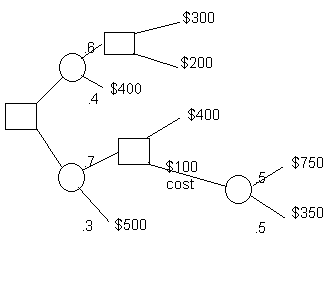
Our first example is given by a typical decision tree diagram. The figure has 12 branches. Profits are to the right of the terminal nodes and notice that there is a $100 cost in the middle for selecting a certain (market research) branch.

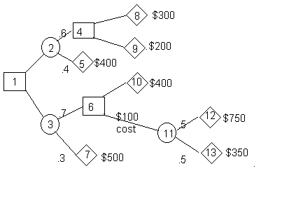
In order to use the decision tree module two things must occur. First, nodes must be added to the right of the ending branches. (Technically, it is illegal to draw a tree that ends with branches rather than nodes). Second, the nodes must be numbered. The figure that follows shows the added nodes and the fact that all nodes have been given numbers.. The most convenient way to number the nodes is from left to right and top to bottom.

The initial data screen is generated by answering that there are 10 branches and that we wish to maximize profits. The following screen contains both the data and the solution.

Start and end node. Branches are characterized by their start and end nodes. An added branch named 'start' appears in order to represent the final outcome. The node values are shown in the far right column. In this example the value of the decision tree is $525.
Branching probabilities. These occur in column 4 and are the probability of going from the start node on the branch to the end node. The probabilities out of an individual chance branch should sum to 1.
Profits or costs. The profit (cost) for each ending node that is terminal is to be entered. In addition, it is possible to enter a profit or cost for any branch. For example, notice that in branch 10 (node 6 to 11) we have entered a cost of $100 by placing -100 in that cell.
The solution data are:
Branch use. For those branches that are decision branches and should always be chosen, an "Always" is displayed. In our example, we should choose (1-3) rather than (1-2). For those branches that we should choose if we get there we display "Possibly". For example, if we get to node 6 we should select (6-9) rather than (6-8). However, there is no guarantee that we will get to node 6 due to the probabilistic nature of the decision tree. The last type of branch is one that we should select if we get there but we should not get there. These are marked as 'Backwards'. Look at branch 7 (node 4 to node 8). If we get to node 8 we should use this branch. However, since we will select 1 to 3 at the beginning we should not end up at node 4.
Ending node. The ending node is repeated to make the output easier to read.
Ending node type. For each ending node the program identifies it as either a final node, a decision node or a chance node.
Expected value. The expected value for each node is listed. For final nodes the expected value is identical to the input. For chance nodes the expected value is the weighted combination of the values of the nodes that follow. For decision nodes the expected value is the best value available from that branch. Both chance nodes and decision nodes will have any costs subtracted from the node values. For example, the value of node 11 is $550. However, the value of node 6 is $450 due to the $100 cost of going from node 6 to node 9.
A graph of the tree structure can be displayed by the program.
